Blur equivalence is a theoretical concept which assigns a precise numerical value to an inherently vague quantity – blur in refractive defocus. The basic premise is simple: overall blur is gauged in terms of equivalence to blur in simple myopia. Thus, if the blurriness of an ametropic eye is no more or no less than an otherwise similar eye requiring -1.00 DS correction, one could state the blur has a unit value of 1.00. In purely spherical refractive errors, this unit is equal to the absolute lens power required to neutralise the refractive error. Hence, the scale for blur equivalence extends from zero in positive numbers only.
(I should emphasise with respect to hypermetropia that it is unaccommodated hypermetropia which will be considered here. Hypermetropia requiring +1.00 DS correction also has an equivalent blur value of 1.00.)
In purely spherical refractive errors, calculation of blur equivalence is trivial. It is only when we come to consider astigmatism that it becomes problematical. For example, what is the equivalent blur in the compound myopic state: -1.00/-3.00 x 180? One can say with certainty the value must be at least 1.00 but no more than 4.00 since those are the minimum and maximum blur values along the principal meridians. Logic dictates that the blurriness of the overall view must lie somewhere between those two extremes, but is it exactly halfway at 2.50?
A simple ‘rule of thumb’ is to add half the cylinder power to the full sphere power (ie to evaluate what is variously known as the ‘mean sphere’, ‘best sphere’, ‘spherical equivalent’). Applying this to the problem above would indeed arrive at a value of 2.50. However, this ‘rule’ does not deliver universally realistic values and must therefore be discarded (for example, the refractive error: +2.00/-4.00x120 would be evaluated as a state of zero blur, which is patently absurd).
So, how can one transform the three numbers associated with a spherocylindrical specification into a single value of blurriness? In actuality, only two of those numbers need be considered since axis is unimportant with respect to overall blur.
Obviously the rule for evaluating blur from sphere and cylinder values must correspond to how blur varies in actuality. In clinical practice visual acuity is our guide to blur, but it is an imprecise measure as it can vary significantly from one individual to another for the same refractive error. However, with a large pool of refractive data it is possible to evaluate statistically how well a presumptive rule correlates spherocylindrical values with acuity and hence infer its validity as a measure of blur.
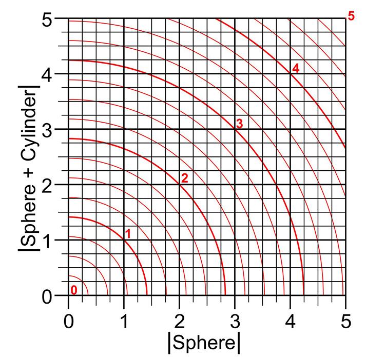
Figure 2: Equivalent blur (red arcs) against principal meridian powers
Thomas W Raasch1 used this approach to analyse the effectiveness of several different calculation methods to predict uncorrected visual acuity from spherocylindrical prescriptions and established which method showed the best correlation between prediction and actual acuity. Figure 1 (equation 1) shows the equation determined by Raasch to give the best fit of E, equivalent blur, to empirical refractive data.
Raasch’s equation can be reconfigured into a form (Figure 1, equation 2) which shows the interrelationship between the principal meridian powers: (Sph) and (Sph + Cyl). From this, a graphical expression of the interrelationship between spherocylindrical refractive errors and equivalent blur can be derived (figure 3). In this graph the absolute values of the principal meridian powers are plotted against each other to reveal the equivalent blur values denoted by the red concentric arcs.
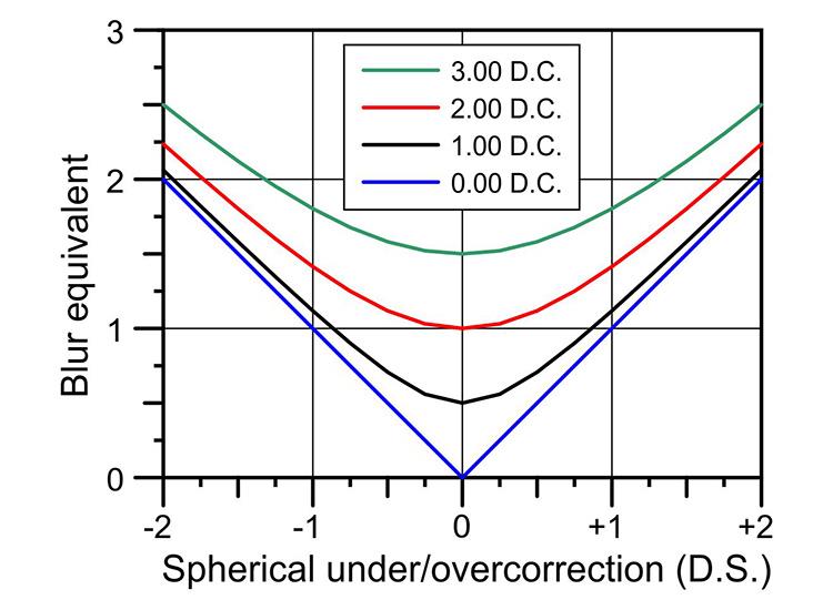
Figure 3: The variation of equivalent blur in various degrees of uncorrected astigmatism
Thus, returning to our specimen refractive error: -1.00/-3.00 x 180, we see the absolute values of the principal meridian powers (1.00 and 4.00) cross between the arcs denoting equivalent blur of 2.75 and 3.00 but closer to the latter, approximately at 2.90. The result by calculation gives a value of 2.915.
What use is all this?
It is always useful to have mathematical models to raise or query theories and hypotheses. For instance: how does blur vary with change of sphere power in uncorrected astigmatism? Figure 3 shows an analysis of this query calculated from Raasch’s equation.
The geometrical basis of blur
Consider a defocused retinal image from a single point object, a bright star in the night sky for example. Assuming a circular pupil, it takes the form of a round patch of light in spherical ametropia. This is known as a blur circle and its diameter is directly proportional to the refractive error (typically a few hundredths of a millimetre per dioptre of defocus).
In astigmatic ametropia the patch of light invariably takes the form of an ellipse (including the circle and line segment as extreme variants). The dimensions of such a blur ellipse are in proportion to the refractive error, the major and minor axes corresponding to the ametropia along the principal meridians.
A blurred image of an extended object consists of an agglomeration of innumerable overlapping blur patches, all the same shape, size and orientation. The puzzle is: what single dimension associated with a blur ellipse is the one corresponding to overall blur?
This author addressed the problem2 and determined that equivalent blur circles and ellipses have the same length of diagonal when either is circumscribed by a rectangle (figure 4). Although compatible with Raasch’s findings, it is not clear how this relates to a consolidation of blur across all meridians.
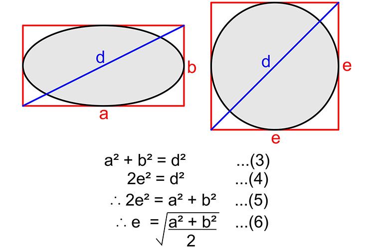
Figure 4: Dimensions of blur ellipse and blur circle of equivalent overall blur
If we consider astigmatic blur in isolated meridians, its maxima and minima occur along the principal meridians, but between those meridians it varies in a continuous manner. Relating this to the geometry of the ellipse there are two dimensions which also vary continuously between the principal axes, the diameter and the width. Although both are the same across the principal axes, their values differ across intermediate meridians of measurement, the width varying in a sinusoidal manner (figure 5).
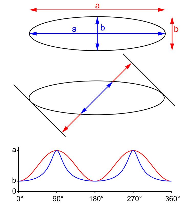
Figure 5: (Upper) Diameter and width of an ellipse. Along the principal axes the diameters (blue) and widths (red) have the same length. (Middle) In other meridians, diameter and width differ. (Bottom) The variation of diameter and width in all meridians. The width varies sinusoidally
It is logical to suppose that overall blur has to be a result of some sort of averaging of blur across all meridians, but which dimension of the blur ellipse is the fundamental one? Diameter? Width? Some combination of both? Neither?
The answer is width. Or to be more specific, it is the root mean square (RMS) width of the blur ellipse. As it turns out, equation 6 (figure 4), gives not only the RMS value of the principal axes, but also the RMS width of the ellipse as a whole.
The root mean square (RMS) width of an ellipse
In principle, to evaluate the RMS width of an ellipse one would need to take width measurements across every possible meridian, square the values, add the squared values together, divide the total by the number of measurements and evaluate the square root of the result.
As there are an infinite number of possible meridians this is clearly a practical impossibility.
Normally, the approach to this sort of problem, dealing with a continuously variable quantity, is to employ integral calculus. However, exploiting a quirk of ellipse geometry makes this unnecessary.
A little known but long-established property of the ellipse is that all mutually perpendicular tangents meet at a fixed distance from the centre of the ellipse. Thus, all perpendicular tangents meet at a circle, known as the director circle,3 which is concentric with the centre of the ellipse.
If a rectangle circumscribes an ellipse, its sides are tangent to the ellipse and its corners lie on the director circle. This results in the extraordinary property that the diagonal length of every possible rectangle circumscribing an ellipse, irrespective of its meridional orientation, is a constant – equal to the director circle diameter (figure 6).
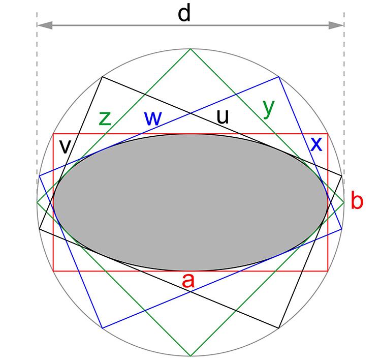
Figure 6: An ellipse circumscribed by four different rectangles. Their side length are a set of perpendicular widths of the ellipse. Although their side lengths differ, the rectangles have the same length of diagonal. The rectangles’ diagonals are diameters of the director circle, diameter d
It should also be appreciated that the side lengths of a circumscribing rectangle are also a pair of perpendicular widths of the ellipse. Thus, perpendicular widths of an ellipse have a Pythagorean relationship with the diameter of its director circle in that the sum of their squares equals the square of the director circle diameter.
Working from basic principles, an approximate RMS width could be calculated from a finite number of width measurements. However, if the measurements are grouped in pairs from perpendicular meridians, the sum of those squared widths always has the same value. Because of this, the calculation of RMS width will always produce the same result irrespective of the number of such pairs sampled (figure 7).
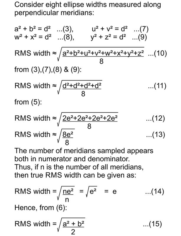
Figure 7: Derivation of ellipse root mean square width
For an exact calculation of RMS width, the width across all meridians has to be taken into account. Since the set of all meridians is also the set of all mutually perpendicular meridians, the exact RMS width of an ellipse must therefore be the same as that calculated from a single pair of mutually perpendicular widths. Hence in equation 6, e is an expression of the RMS width of an ellipse.
Conclusion
The dimension of a blur ellipse which corresponds to overall blur is its root mean square width. And, by extension (cf equation 2), overall blur in astigmatism is the root mean square of blur in all meridians.
Henry Burek is an optometrist practicing in South Yorkshire and an examiner for the College of Optometrists.
Acknowledgements
My thanks to Professor David Elliot of the University of Bradford, UK, for his invaluable assistance.
References
1 Raasch TW. (1995). Spherocylindrical Refractive Errors And Visual Acuity. Optom Vis Sci. 72, 272-275
2 Burek H. (1999). How Blurred Is Blurred? Optician. 217. January 15th. 2426
3 Daintith J & Nelson, RD. (1989). The Penguin Dictionary Of Mathematics. Penguin Books, London. Pg 100