Progressive power lenses are designed to provide continuous vision at all distances instead of the predetermined working distances of a bifocal or trifocal design. A progressive lens can be considered to have three zones, just like a trifocal lens; a distance zone, a progression zone, and a near zone (figure 1). Unlike a trifocal lens, however, the power of the lens increases over the progression zone from the distance power at the top to the near power at the bottom (figure 2).
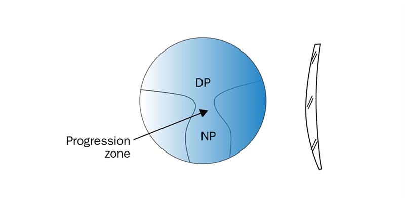
Figure 1: Progressive power lens
The difference in power distribution between an E-style trifocal lens and a progressive power lens is shown by the graphical plots in figure 2, which indicate how the power varies from the top to the bottom of each type of lens. The variation in power along the vertical meridian of the lens is usually illustrated graphically, as shown in figure 2. The two graphs compare the discrete power areas of a trifocal lens (2(a)) with the gradual increase in power of a progressive lens (2(b)) from distance to near. The term power variation lens is sometimes used to describe these lenses.

Figure 2: Comparison of power variation for E-style trifocal and progressive lens
a) Power variation from top to bottom of an E-style trifocal lens made to the specification
+2.00 Add +2.50 for near, 50% IP / NP ratio.
b) Power variation from top to bottom of a progressive lens made to the specification
+2.00 Add +2.50 for near, 15mm progression length.
In the case of the trifocal lens (figure 2(a)) the DP power is +2.00 D, the IP power is +3.25 D and the NP power is +4.50 D. The lens diameter is 60mm and the IP is 15mm deep. In the case of the progressive lens (figure 2(b)), the DP power is +2.00 D and the NP power is +4.50 D, but between the DP and NP, the power increases from +2.00 D to +4.50 D at a steady rate.
The progressive power design shown in figure 2(b) is said to have a linear power law since the power increases at a steady rate over the progression zone from distance to near. The power law expresses, mathematically, the rate at which the power increases from the top to the bottom of the progression zone. In the case of the simple linear power law, which is illustrated in figure 2(b), if the addition is denoted by A and the depth of the progression zone by h, then the increase in power per millimetre through the progression zone, δA, is given by
 For the design illustrated in figure 2(b), the length of the progression zone is 15mm and the add is +2.50 D, so the power is increasing throughout the zone by
 where f(A) can often be expressed in terms of a quadratic or trigonometric function of the add.
For example, it is seen in figure 3 that, for a typical modern design, the power actually begins to increase from a point about 4mm above the designated start point for the progression and begins to decrease again below the end of the progression corridor.
Other features of the power law of progressive power lenses can be deduced from figure 3. The red dashed line represents the path which would be taken by a design with a linear power law of 20mm depth and it can be seen that there is a slower increase in power in the upper part of the progression zone which becomes more rapid towards the end of the progression.
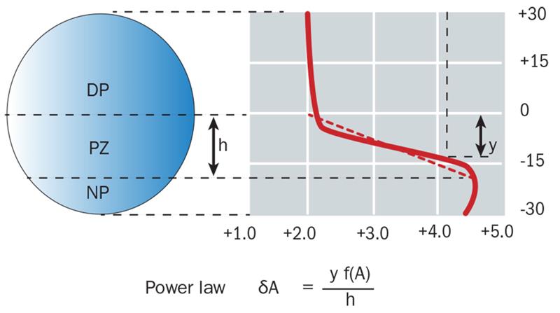
Figure 3: Power variation from top to bottom of a progressive lens with a non-linear power law made to the specification, +2.00 Add +2.50 for near, 20mm progression length
Many modern progressive lenses are designed such that at least 85% of the addition is obtained some 12mm below the start of the progression, which for the +2.50 Add depicted in figure 3, is 0.85 x 2.50 = +2.12 D. This value has been achieved at a point, y mm below the geometrical centre of the lens in the figure, where y is seen to be 12mm.
Modelling the progressive surface
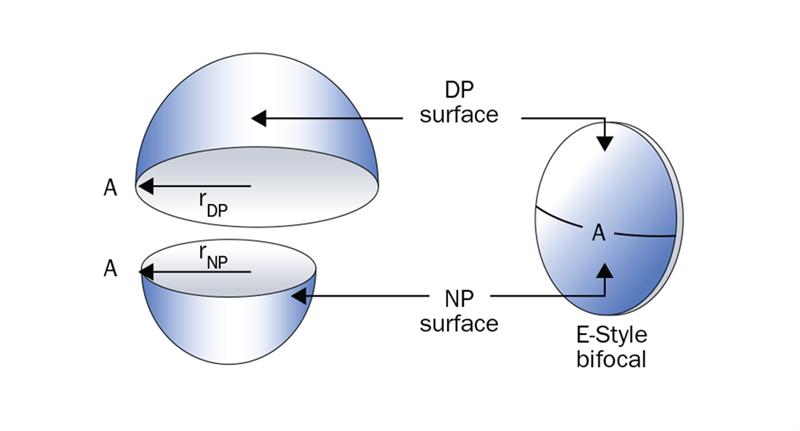
The principle of the progressive surface can be understood by considering the geometry of a simple bifocal lens, such as the E-style design shown in figure 4. The bifocal surface is formed from two spherical surfaces of different radii of curvature, the surface of the longer radius forms the distance portion (DP surface), and the surface of the shorter radius forms the near portion (NP surface). When these two surfaces are put together to form the bifocal surface, although they share a common tangent at A, there is a mismatch between the surfaces. This gives rise to a visible step at the dividing line, of increasing depth on moving away from the vertex, A. Normally, the lens diameter is small compared with the radii of the surfaces and the step between the two surfaces is small.
In order to make a progressive lens, the two spherical surfaces must be connected by a third surface whose radius decreases at a continuous rate from that of the DP, to that of the NP. What form does this surface take? There must be no visible dividing line, so the DP and NP must be connected by a zone whose power increases at a continuous rate from that of the DP surface, to that of the RP surface. In other words, the radius of curvature must decrease at a continuous rate from the DP to the NP.
Such a surface can be found on an oblate ellipsoid, or, some higher-order aspherical surface based upon this shape. With this surface, which is depicted in dashed outline in figure 5, it can be seen that the sagittal radius decreases on moving away from the vertex along the tangential meridian of the surface. It will be realised that if the oblate ellipsoid is chosen such that its vertex radius at A, (rDP), exactly matches the radius of the hemisphere which represents the spherical distance portion, and that the lower edge of the section is chosen such that its sagittal radius at N, (rNP), exactly matches the radius of the hemisphere which represents the spherical near portion, then when these three components are placed together, an ovoid shaped solid will be obtained which has no discontinuity in its surface.
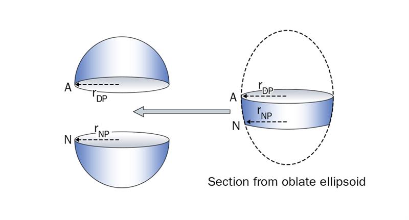
Figure 5: Modelling the progressive zone with a section taken from an oblate ellipsoid
Suppose that a lens measure reads +6.00 D when placed along the vertical meridian of the oblate ellipsoid with its central leg at point A. If the lens measure is slid down the surface so that its central leg lies at point N, it might now read +8.00 D, in which case the surface has increased in power by +2.00 D, ie provided an addition of +2.00 D. It is quite clear that the surface curvature in the tangential meridian increases from A to N at a steady rate.
The p-value of the conicoid that will produce a given near addition, A, over a progression zone of depth, y mm, can be obtained from the Davis-Fernald relationship,2 which gives the p-value for a conicoidal surface which is required to eliminate tangential error, δT, at a point y mm from the pole of the surface. In the case of a progressive lens, a tangential error is required which is equal to the near addition, A. Assuming that the progression is to be formed on the front surface of the lens, then the asphericity can be found from the equation.2
p = 1 + (r1/y1)2.{1 - [F1/(F1 + A)] 2/3}
This relationship, which gives the required value for p, provides some preliminary information from which the design of the tangential meridian of the progressive power surface might begin.
In the case of a +6.00D surface worked on a material of refractive index 1.50, an add of +1.00 at 15mm below the pole of the surface would require an asphericity of +4.0. For an add of +2.00 the surface would require an asphericity of +6.4 and for an add of +3.00, an asphericity of +8.3. These p-values describe oblate ellipsoidal surfaces such as the one depicted in figure 5.
Figure 6 shows that the progression zone can be likened to a section of an oblate ellipsoid which increases in power from the distance reference point, A, to the near reference point, N. The line joining these two points, has been called the meridian line. Assume for the time being, and from a theoretical point of view, that above A, and below N, the surface remains spherical. The dashed circular arcs shown in figure 6, whose radii are given as rD and rN respectively, are traces of the spherical surfaces representing the distance and near portions of the lens.
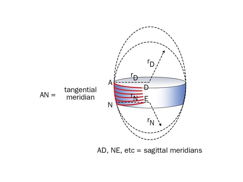
Figure 6: Tangential and sagittal meridians of progressive zone
The power variation for an oblate ellipsoid along the meridian line, AN, is shown in figure 7(a). The power of the lens is +2.00 add +2.00 for near, and it is seen that in the tangential meridian, the lens increases in power from +2.00 D at point A in the distance portion, to +4.00 D at a point, N, some 15mm below A. However, the ellipsoidal surface is astigmatic and when the sagittal meridians between A and N on the surface are considered, it can be seen that the sagittal curvature hardly changes at all (figure 6). At the bottom of the progression zone, where, ideally, the power should be +4.00 D sphere, the graph in figure 7(a) shows that the power is actually +4.00 in the tangential meridian and +2.62 in the sagittal meridian, ie the power along the meridian line as the eye enters the near portion is +4.00 / -1.37 DC.
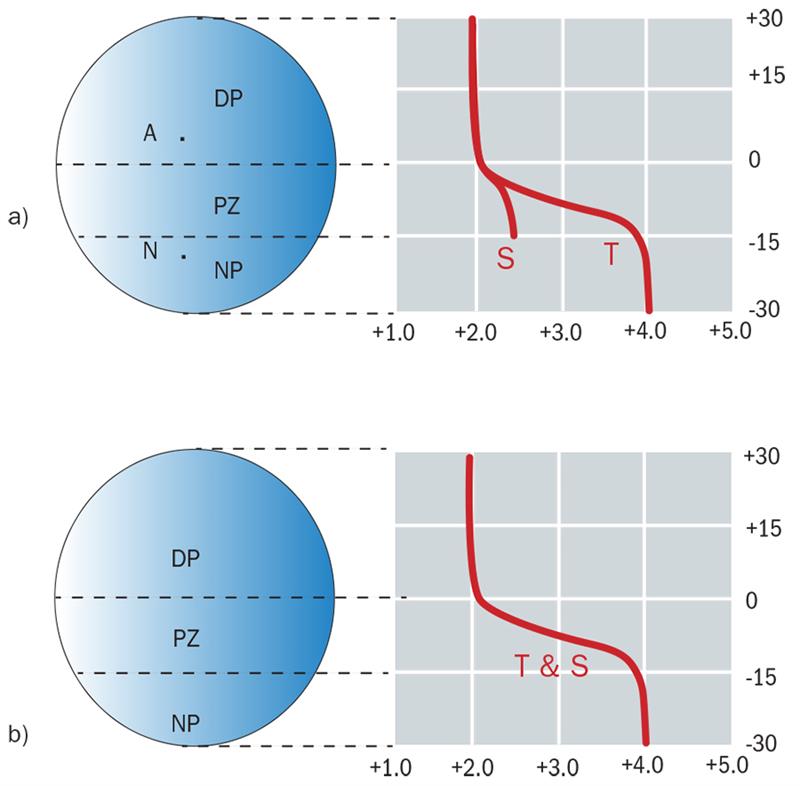
Figure 7: Variation in astigmatism along the meridian line before and after correction of the sagittal curvatures between points A and N
a) Tangential, T, and sagittal, S, plots along the meridian line of progression zone when a simple oblate ellipsoid surface is used.
b) T and S equalised along the meridian line of progression zone by increasing the sagittal curvature between A and N.
The amount of astigmatism which occurs as the eye moves down through the progression zone is easy to calculate along the meridian line and knowing this, the designer can increase the sagittal curvature, point by point between A and N along the meridian line, to eliminate the astigmatism along this line, as shown in figure 7(b).
The change in sagittal curvature must be gradual as the eye moves through the progression zone, particularly in the peripheries of the progression and near zones of the lens, and it is mainly this feature of the surface which differentiates the various progressive designs which are available.
Production of the progressive surface
Complex lens surfaces such as the progressive surface, are produced by computer numerically controlled (CNC) grinding machines where a single point cutter, under computer control, traverses the lens surface. With modern CNC machining processes the (x,y,z) data for the progressive surface is stored in data banks and is available to be called by the on-board computer, to generate the surface.
If a simple convex or concave progressive surface is to be produced, then surface data will be held in separate files for each eye, base curve and near addition, and if the design is available in different refractive index materials, then separate files will be held for each medium. Typically, for any given design, in a given refractive index, and a range which comprises three different base curves and 12 near additions, manufactured for both right and left eyes, a total of 144 different semi-finished blanks must be stocked by the surfacing laboratory to cover any possible demand for a pair of lenses.
An extract from the contents of a typical data base for a convex progressive surface is illustrated in figure 8 which is a topographical representation of the surface. The (x,y) values step in 5mm intervals and the z-values shown cover a surface of diameter 60mm, with a +4.00 D base curve and +2.00 addition, worked on a plastics material of refractive index, 1.662. In practice, to generate the surface, the (x,y) intervals would need to be much smaller, typically the step interval would be in the order of only 0.50, or even, 0.25mm.
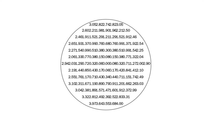
Figure 8: Free form description of a convex progressive power surface (From US Patent 6 049 470 : February 2000, H Mukaiyama & K Kato, Patent assigned to Seiko Epson. Japanese application dated November 24 1995)
The z-values given in figure 8 for (x,y) = (±5,+20) are each 1.29mm and assuming that the surface in this region of the DP surface is spherical, the tangential power of the surface at these points is given by
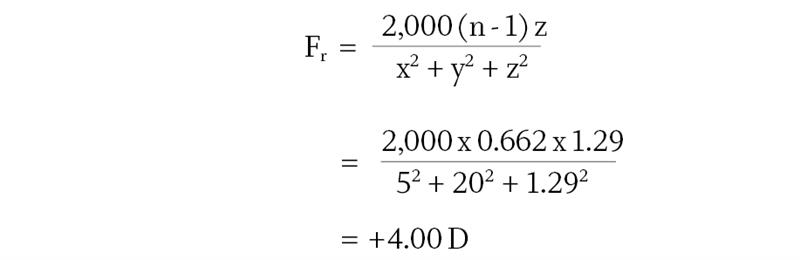
This method can be used to determine the physical shape of the DP surface from its (x,y,z) description.
Evaluation of the curvature along the meridian line is strictly only valid for a progressive surface whose power law follows that provided by an ellipsoid of the computed asphericity. However, it should be remembered that the tangential power at any point is a function only of the tangential radius of curvature at that point and the refractive index of the material upon which the surface has been worked, ie, FT = (n - 1)/rT. In the simplest of terms, the progressive surface designs from various manufacturers really differ from one another, only in the manner in which the manufacturer has chosen to vary the tangential and sagittal radii of curvature at points in each zone of the lens. For a given power law and progression length, the tangential power along the meridian line, at least, must vary as depicted by the power law. In other words, if the tangential power at some point on the meridian line is +5.00, then the tangential radius at this point must be (n - 1)/5.00 metres.
Figure 9 illustrates the paths of the horizontal raster cuts produced by the cutting tool as it moves down the surface from the top to the bottom of the lens. In the DP zone the tool sweeps out circular paths. Through the progression zone, the cuts become progressively steeper in the central zone to eliminate the astigmatism along the meridian line. Along the meridian line, the surface curvatures in the sagittal plane have been made to match the surface curvatures in the tangential plane, point by point along the surface. The meridian line has thus become an umbilic line for the surface.
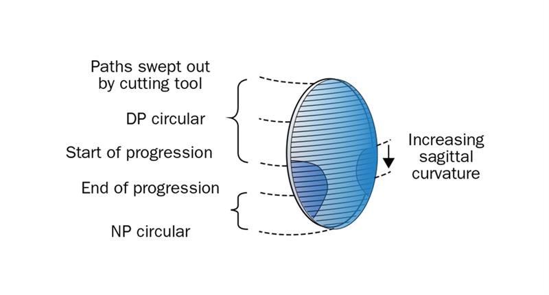
The shape of the section, however, is no longer a simple section of an oblate ellipsoid. It might even become concave towards the periphery of the zone in order to blend the surface to the designer’s requirements. In the near zone, the horizontal sections again become circular. It will be realised that, in order to connect the zones together smoothly, some optical discontinuity will occur in the progressive surface, particularly towards the edges of the lens where the distance zone meets the upper region of the progression zone and the lower region of the progression zone meets the near portion. The zones of discontinuity are shown as the shaded areas at the peripheries of the progression in figure 9 and result from the blending of the surfaces to form smooth transitions between the various zones of the surface.
Early progressive lenses prioritised clear vision in the distance portion concentrating the blending at the bottom of the progression zone where it becomes the near portion (figure 10(a)).
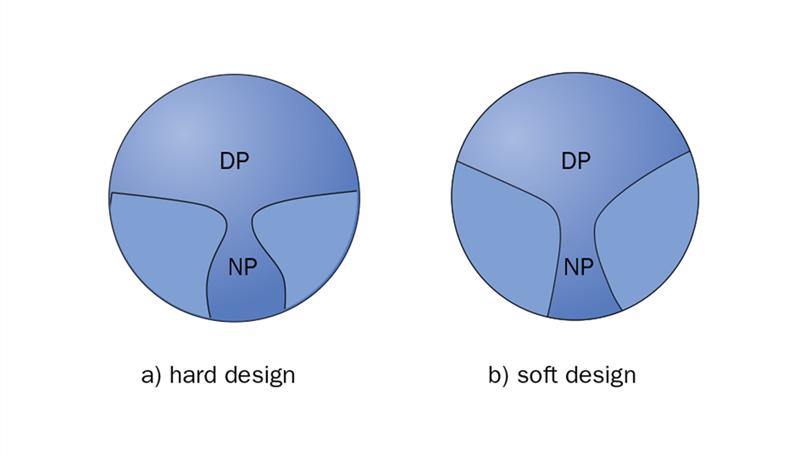
Figure 10: Progressive design philosophies
This form of blending allows a wide distance zone, but results in large discontinuities in the lower nasal and temporal regions of the surface. Such designs have been called ‘hard’ progressive designs.
Alternatively, the blending can be extended into the distance area of the lens which reduces the discontinuities between the bottom of the progression zone and the near portion but transferring it to the distance zone (figure 10(b)). Such designs have been called ‘soft’ progressive designs and, without doubt, it was the introduction of soft designs with their lower levels of surface astigmatism that enabled subjects to adapt to progressive lens wear more rapidly.
Early CNC generators which were first used in the ophthalmic lens industry were relatively slow compared with today’s high speed cutting and polishing machines and some manufacturers introduced a vacuum forming process from which they could slump several finished glass progressive surfaces from one ceramic mould, or produce glass moulds from which plastics lenses could be cast.
The vacuum forming, or slumping, process is illustrated in figure 11. First, a ceramic mould is produced by CNC generating of a refractory ceramic block, the surface being carefully calculated to take into account the deformation in the surface which will occur during the slumping operation.
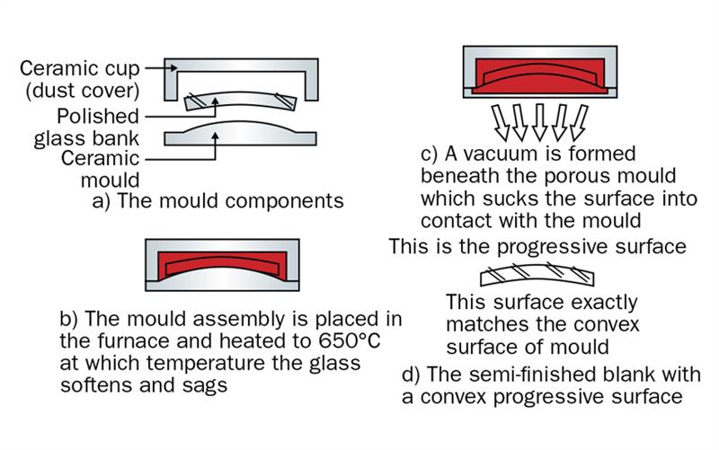
The generated surface has a very smooth finish. A glass blank is then very carefully surfaced on both sides to predetermined curves and polished to a high degree of accuracy, to ensure that the surfaces are of precise spherical form. The glass blank is placed on the mould, very carefully cleaned and the assembly covered with a ceramic cover to ensure that no dust or other foreign particles can spoil the surface (figure 11(a)).
The assembled moulds are placed in a furnace and the temperature raised over a four hour period to about 650°C when the glass blanks begin to soften and sag onto the ceramic moulds (figure 11(b)). This temperature is maintained over a period of about one hour during which time the sagging process is assisted by applying a vacuum under the porous moulds which effectively sucks the blanks onto the convex surfaces of the moulds (figure 11(c)). The temperature is then reduced in an annealing period of about eight hours.
The finished glass blank is shown in figure 11(d). The desired surface shape on the convex surface of the ceramic mould has been transferred to the convex side of the glass blank, the concave side of the blank bearing the surface finish of the convex surface of the ceramic mould. If a glass lens is to be produced by the process, the concave surface would be completed in the same way as a semi-finished lens. If a mould from which plastics lenses may be cast is to be produced, then the ceramic mould will have a concave surface into which the glass blank will be sagged.
Optics of the progressive surface
Figure 12(a) illustrates a narrow pencil of rays incident upon a progressive lens at some point, P, in the progression zone, P lying close to the meridian line, and the ray diagrams in figures (b) and (c) show the form of the refracted pencil before it enters the eye. Assume that point P has co-ordinates (x,y) and that it lies at the centre of the small zone, on the lens through which the narrow pencil passes whose diameter is d. The surface power for the ray passing through the upper edge of this zone, whose ordinate is y – d/2, has been denoted by F.
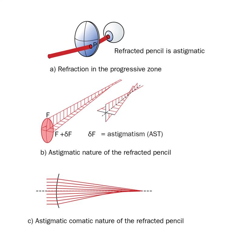
Figure 12: Form of the pencil resulting from refraction in the progression zone
Since the surface is progressive, the surface power must have increased for the light which passes through P, by the quantity, δF, which represents the astigmatism, (AST) for the surface at P. For example, if the tangential power of the surface at the upper edge of the zone is +5.00 D (so that F = +5.00), and the full near addition, A, is +2.00 D, the progression zone having a depth of 16 mm, with a linear power law, the surface power increases at the rate of 2/16 D per mm, ie, by 0.12 D per mm. If the diameter of the zone is assumed to be 4mm, the tangential power of the surface at the centre of the zone must have increased to +5.25 D and the sagittal fan of rays will meet the axis closer to the surface than the ray incident at the top of the zone (figure 12(b)).
Clearly, the surface is astigmatic, and the ray passing through the top of the zone will meet the auxiliary axis at the distance n/F metres from the surface, whereas sagittal rays meeting the surface at the centre of the zone will focus at n/(F+δF) metres from the surface. The refracted pencil, however, is not identical to Sturm’s Conoid, since the rays arriving below P, will focus closer and closer to the surface. For example, at the bottom of the zone the lowest ray will meet the axis at n/(F+2δF) metres from the surface. The effect is similar to that of tangential coma across the zone (figure 12(c)) and the narrowest area of the pencil in the region of the focus is an ellipse. Except along the umbilic line where most designers aim to eliminate astigmatism, at any other point on the progressive surface, the tangential power, FT, and the sagittal power, FS, are unequal and the surface has astigmatism, AST, at the point in question, given by
AST = FT - FS
At the same point, the mean surface power, M, is given by

It follows from these two expressions that
FT = M + AST / 2 and FS = M - AST / 2
As previously noted, along the meridian line of the surface, the astigmatism is normally eliminated, so that FT = FS = M.
At some point P(x,y) close to the meridian line,
FT(x,y) = M(y) + x A(y) / h
and FS(x,y) = M(y) - x A(y) / h
where A(y)/h is the rate of change of addition, A, per millimetre, at y mm below the start of the progression, whose full depth is h, and the astigmatism at the point

This expression is often referred to as the Minkwitz Rule since it was first pointed out by the German scientist, G Minkwitz3 that if a surface increases in power along an umbilic line, then the surface is afflicted with astigmatism which increases at twice the rate of change, (ie 2A/h D per millimetre), at right angles to the umbilic line. The surface astigmatism is an inevitable consequence of a progressive surface. The Minkwitz Rule shows us that the surface astigmatism increases as the near addition, A, increases and as the progression depth, h, decreases. From the wearer’s point of view, the degree of surface astigmatism should be kept as low as possible, in order to provide the widest intermediate and near fields of clear vision and to allow rapid adaptation to the design. If no blending or softening of the design were to take place then the Minkwitz rule would result in a contour plot similar to that shown in figure 13. Such hard designs where the astigmatism might have reached as much as 10.00 D, have proven not to be acceptable to most wearers, long periods of adaptation being required to become accustomed to the rapid movements caused by the astigmatism in the periphery of the lens.
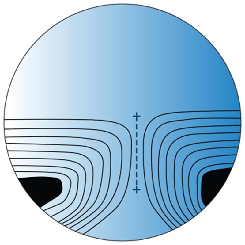
Figure 13: Minkwitz astigmatism
For a progressive lens with a near addition of +2.00 D and a 16mm progression depth, the distance from the umbilic line to the 0.25 D iso-cylinder line, from the Minkwitz Rule, would be

and the total width of the corridor where the astigmatism is less than 0.25 D is 2mm. The width of the corridor where the astigmatism is less than 0.50 D is 4mm and so on.
Typical contour plots for two modern progressive lens designs showing the result of reducing the curvatures in the peripheries of the progression and near zones are illustrated in figure 14. The iso-astigmatism lines are plotted in 0.50 D intervals and the astigmatism is seen to increase rapidly as the eye moves towards the edges of the progression and near zones of the lens. The effect of the astigmatism is to produce a corridor of clear vision, the actual shape of which depends upon how the designer has chosen to blend the various powers together towards the edges of the lens.
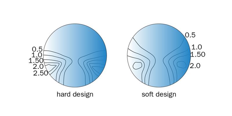
Figure 14: Minkwitz astigmatism for modern progressive designs
By considering that the blending process is that of blending the dividing lines together, some idea of the zones of the lens where the vision will be poor can be obtained. The zones where the blending occurs, depends upon the designer’s concept of how the power changes should occur across the surface. Figure 15 illustrates two different concepts which have been used as the basis of progressive design with a plano distance portion and near addition of +2.00 D.
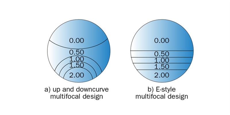
Figure 15: Power distribution for the progressive surface
In figure 15(a), the designer has selected an upcurve bifocal with a large segment to form the DP, and a series of concentric downcurve segments to provide an ever-increasing series of additions until the full near addition is reached. The design can be looked upon as an upcurve bifocal made to the specification, +0.50 D add -0.50 D for distance and each downcurve segment adds +0.50 D to the previous segment to achieve the powers shown in each region of the lens. In figure 15(b), the designer has chosen an E-style multifocal concept with each segment band adding +0.50 D to the previous band.
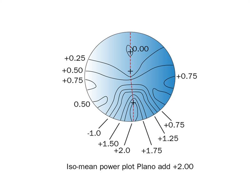
Figure 16: Iso-mean power plot for specification plano add +2.00
This concept illustrates how the mean power varies across the progressive surface. This can be shown either by a contour plot of the mean power, an iso-mean power plot, or by means of a plot which shows how the power varies from the desired power of the surface, an iso-mean power error plot for the design. An iso-mean power plot for a design based upon the up and downcurve concept illustrated in figure 15(a) is illustrated in figure 16. Note that the iso-mean power contours represent the quantity, M, where

The dashed red line represents the meridian line for the progressive surface and the upper cross in the distance portion represents the position of the distance design reference point, the lowest cross in the near portion represents the near design reference point and the cross near the centre of the lens represents the position of the fitting cross, which is normally fitted so that it lies in front of the centre of the wearer’s pupil. It can be seen that one criterion which has been chosen for this lens is to soften the design, by reducing the mean power of the progressive surface as the eye rotates horizontally in the progressive and near regions of the surface. This is shown quite clearly in figure 17 which shows the variation in power along a horizontal line which has been drawn through the near design reference point.
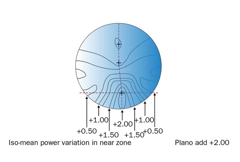
Figure 17: Iso-mean power plot showing softness of the design in terms of power reduction
An iso-mean power error plot is obtained by comparing the design concept with an iso-mean power plot to show the areas of the lens where the powers depart from the design concept. In figure 18(a), the iso-mean power plot for the lens, plano, add 2.00, which is shown in figure 16, has been superimposed upon the design concept illustrated in figure 15(a) (reproduced with the fine dashed red lines). The interval between the different zones has been reduced to 0.50 D steps for clarity.
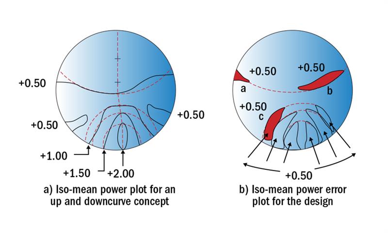
Figure 18: Iso-mean power error plot for specification plano add +2.00
The information provided by the iso-mean power error plot shown in figure 18(b) can be obtained as follows. In the zone marked (a) the power which is required in the design concept is +0.50 D (see figure 15(a)), but the +0.50 D iso-mean power contour has not yet been reached in that area of the lens, so that the error is up to -0.50 D. In the zone marked (b), the power required is plano but in fact the power has already increased to +0.50 D, which is the error shown for this zone. By the same reasoning, for the zone marked (c), the power required is +1.00 D but it is still only +0.50 D, so the error is -0.50 D and so on. It will be realised that each successive fang-shaped zone surrounding the near portion is -0.50 D weak, when compared with the design concept.
In addition to the asymmetric astigmatism inherent in a progressive power lens, there must also be skew distortion inherent in the surface, which arises as follows. Suppose the eye is viewing three vertical lines through a bifocal lens, held at arm’s length, the flat-top bifocal design having the power, plano, add 2.00 D. Since the power is greater in the near portion, the magnification of the lines is also greater in the near portion and the appearance would be as shown in figure 19(a). However, since the addition is constant over the whole of the near portion, the magnification is also constant and the three lines still appear to be vertical when viewed through the near portion.
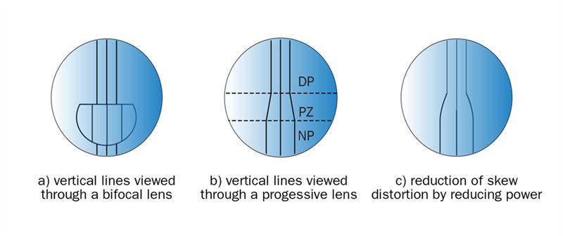
Figure 19: Skew distortion exhibited by a progressive lens
Now consider what must happen when the lines are viewed through a progressive lens (figure 19(b)). Over the progression zone, the power of the surface increases from that in the distance portion to that in the near portion, so the magnification must also increase at the same rate. It should be obvious that there cannot be an increase in power without an accompanying increase in magnification.
Thus, viewed through a progressive lens, the variation in magnification indicates that vertical lines appear to slant. This variation in magnification is sometimes noticed by spectacle wearers when given their first pair of progressive lenses, who describe it as a swimming effect.
Fortunately, the skew distortion of vertical lines can be minimised by deliberately reducing the power and, therefore, the magnification, in the lateral regions of the progression zone, and owing to the plasticity of the visual system, the swimming effect soon disappears. It can be seen from the iso-mean power plot illustrated in figure 17 that this is just what happens in a typical modern progressive power lens. The resulting effect is to cause the change in direction of the lines to take place more gently as shown in figure 19(c).
Prism thinning
It can be seen from a vertical cross-section of a progressive lens (figure 20(a)), that the edge thickness of the lens is greater at the top edge of the lens (tE90), than at the bottom edge (tE270). This occurs because the curvature of the surface increases towards the bottom of the lens by the magnitude of the near addition. As a result, the centre thickness of a plus lens needs to be greater than that based upon the distance prescription alone. By incorporating base down prism in the lens (or removing base up prism across the lens), the edge thickness can be equalised at its top and bottom edges.
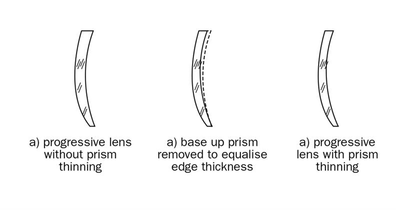
Figure 20: Thickess reduction prism or prism thinning
This addition of thickness reduction prism (prism thinning) to the lens, enables progressive lenses to have a smaller centre thickness than when prism thinning is not applied. The same amount of thickness reduction prism is incorporated in each lens and, typically, the amount of prism is equal to two-thirds of the near addition with its base at 270°. For an addition of 1.50 D the reduction prism would be 1Δ, for an addition of 2.00 D the reduction prism would be 1.33Δ and so on. This small amount of base down prism has virtually no effect upon the quality of vision.
When verifying progressive power lenses, prism thinning, when included, must be taken into account when establishing the prismatic effect exerted by the lens. Prism power is usually checked at the geometric centre of the lens and in the absence of any prescribed prism, only prism thinning would be read at this point. If no prism thinning is supplied, then the optical centre would coincide with the geometrical centre.
Whether or not to incorporate a thickness reduction prism depends upon the power and shape of the finished lens. For example, the combination of both a shallow lens shape and a low progression depth would place the geometrical centre of the uncut nearer to the bottom edge of the lens and prism thinning would have little influence over the thickness (figure 21). Furthermore, many surfacing laboratories do not apply any thinning prism to strong minus lenses.
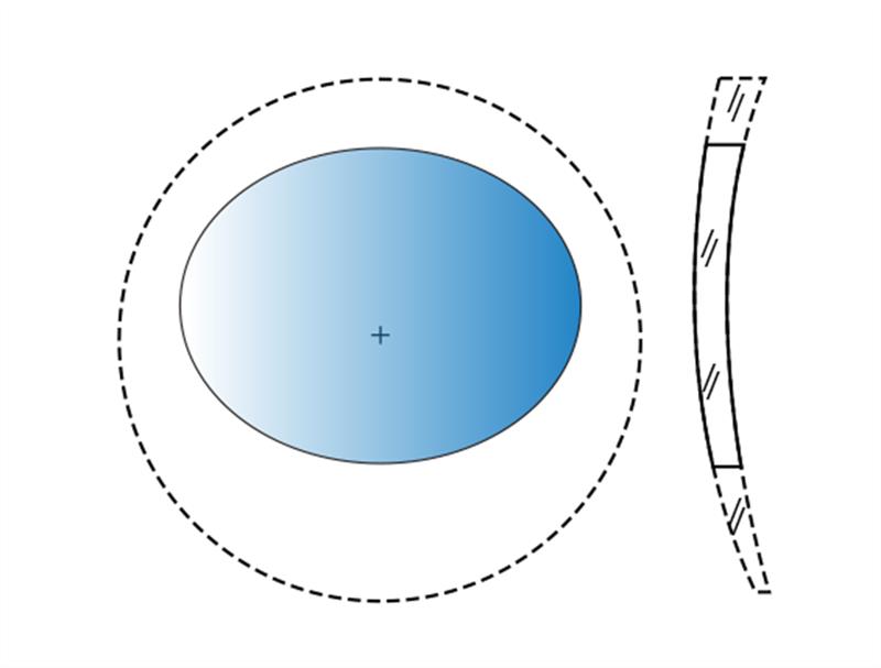
Figure 21: Shallow lens shape without prism thinning
Prismatic effects in the progression zone
Figure 22 illustrates a ray of light incident at a point, D, on the meridian line of a progressive power lens at a distance y cm below the prism reference point, A1, of the lens. It is assumed that the optical centre of the distance portion lies at this point (ie no thinning prism has been applied to the lens). The slope angle of the incident ray is denoted by u and it is assumed that the instantaneous power, FT, is known at the point, D. This value can be ascertained from knowledge of the power law for the surface, as shown in figure 3, or read from an iso-mean power plot for the surface. The ray is refracted at D and the refracted ray makes an angle u' with the axis. The deviation of the ray, P, expressed in prism dioptres is u' - u.
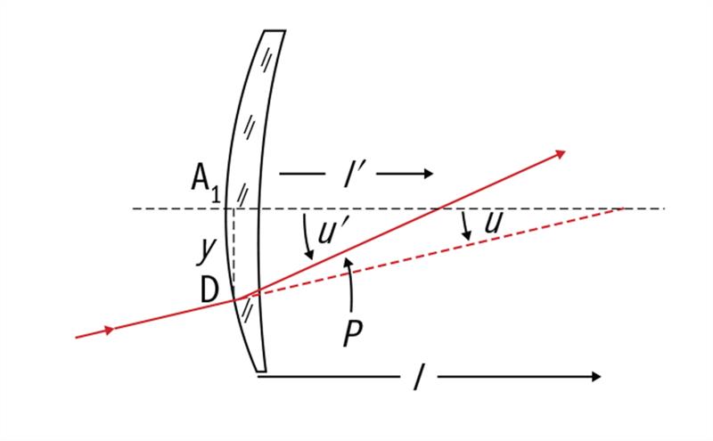
Figure 22: Prismatic effect along the meridian line of a progressive lens
From the definition of the prism dioptre,
u = 100 y / l = y L (l expressed in centimetres)
u' = 100 y / l' = y L' (l' expressed in centimetres)
so P = u' - u = y (L' - L) = y FT
This, of course, is Prentice’s Law. The derivation assumes the use of paraxial theory, which gives a good approximation to the true deviation of the tangential ray at the point of incidence. If the meridian line is an umbilic line (so that FT = FS), then the prismatic effect is simply, P = y F where F is the instantaneous power of the surface at the point in question, as might be read from a graph showing the power law for the surface in question, as illustrated in figures 2(b) and 3.
Compared with bifocal and trifocal designs the progressive power lens provides four important advantages. First, it provides continuous vision from the far point to the near point with no gaps in the range of vision (figure 23(b)).
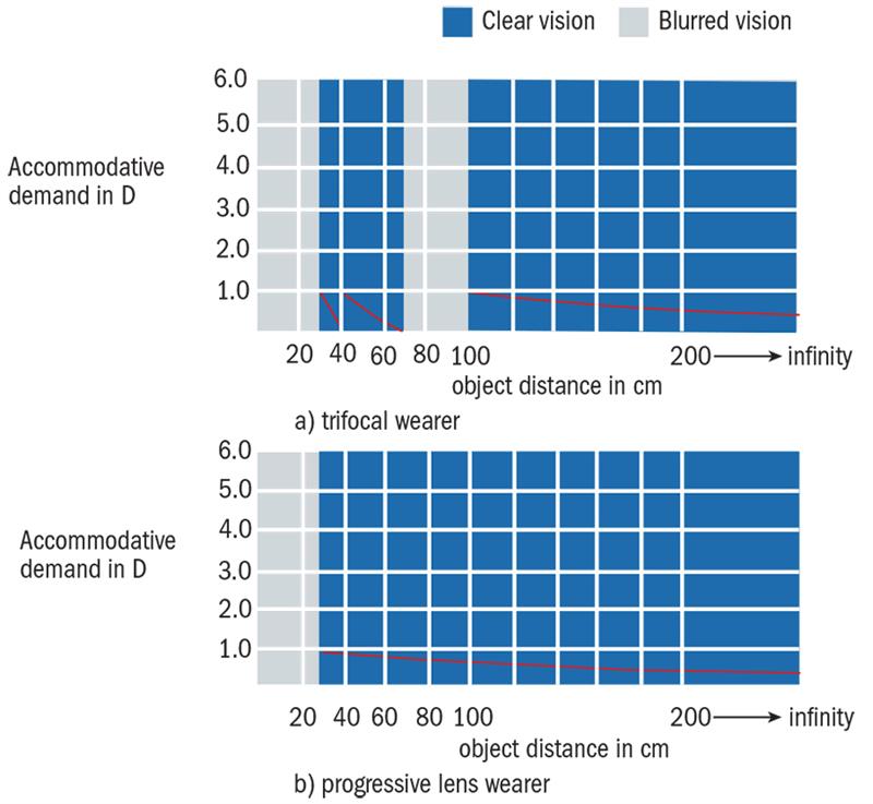
Figure 23: Comparison of accommodative demand with trifocal and progressive lens wear
Secondly, use of the remaining accommodation is more natural, since the accommodative demand increases gradually, as it did before the onset of presbyopia. This feature is illustrated in figure 23 which compares the accommodative demand for a subject who possesses a total amplitude of +1.00 D, wearing a) trifocal lenses, b) progressive lenses. Note the fluctuation in accommodation required by the trifocal lens wearer, which disappears when progressive lenses are worn.
A third advantage is that there is no image jump, since there is no sudden change in power between the various zones. Finally, there is no visible dividing line on the progressive surface. The lens has the outward appearance of a single vision lens.
Professor Mo Jalie is a visiting professor at Ulster University and author of the new edition of Principles of Ophthalmic Lenses.
References
1 Jalie M (2016) Principles of Ophthalmic lenses, 5th Edition, Abdo.
2 US Patent 3960442 (1976) Davis JK, Fernald HG. Ophthalmic Lens Series.
3 Minkwitz G (1963). On the surface astigmatism of a fixed symmetrical aspheric surface. OptActa (Lond), 10:223–7.