The iso-astigmatism and iso-mean power plots of typical progressive power lenses represent the effects of Minkwitz astigmatism and the method chosen by the manufacturer to blend the distance, intermediate and near zones together. They can be looked upon as ‘fingerprints’ which are helpful in explaining the main design characteristics of a progressive lens. In particular, their positions immediately inform upon whether the design is hard or soft as depicted in figure 1.
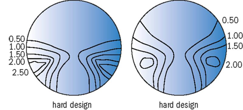
Figure 1: Minkwitz astigmatism for modern progressive designs
These plots are frequently given to identify the characteristics of the various designs. However, it should be borne in mind that they often represent the characteristics of a single surface, normally chosen for the prescription, plano, add +2.00 D, in which case the DP curve is in the region of 5.50 to 6.50 D (figure 2) and the back surface, or prescription surface, is assumed to be spherical.

Figure 2: Typical surface powers for a semi-finished blank for the prescription plano add 2.00
As will become apparent, the contour plots do not show the effects of the total astigmatism and distribution of mean power when the surface is used for prescriptions other than that for which the surface was designed. The commonest method for producing these plots, in practice, is by means of reflection deflectometry, that is, by measuring the reflected light pattern from a specular surface to calculate its shape. Several instruments such as the Rotlex Class Plus1 spectacle lens inspection system (Israel) and the Automation & Robotics Dual Lens Mapper2 (Belgium) are available for doing this, in addition to smaller Automatic Lens Analysers such as the Visionix Wave Lens PRO Lensometer3 based on Hartmann-Shack wave front analysis. These instruments provide high-resolution power and astigmatism maps, which are used for verifying the prescription, assessing the design and finding production-related defects.
The Rotlex Class Plus, was developed from the OMS 400 instrument, one of the first lens mapping instruments to use Moiré deflectometry. Lens mappings obtained from the Rotlex Class Plus instrument are illustrated in figure 3 which show iso-astigmatism and mean power plots for a typical progressive power lens.

Figure 3: Iso-astigmatism and iso-mean power mappings for a progressive lens from Rotlex Class Plus
Although the mappings are not able to predict wearer acceptability of any particular progressive design, it has been suggested4 that they are useful for grading progressive lens performance by considering various characteristics which can be deduced from the plots. Figure 4 repeats the mappings shown in figure 3 to a larger scale showing only the relevant zones from which these characteristics can be deduced.

Figure 4: Interpreting information from a contour plot
The criteria which follow have been proposed by Dr Raanan Bavli, R&D manager at Rotlex, as being the most useful method to assess the information which is obtained from a contour plot.
In figure 4, points A and B on the iso-astigmatism plot represent the points in the intermediate zone where the Minkwitz astigmatism has reached its maximum value on either side of the corridor. The symmetry of the design can be expressed, quantitatively, by the expression
FA - FB
where FA represents the value of the astigmatism at point A and FB represents the value of the astigmatism at point B. Good designs have symmetry values less than 0.05.
The amount of astigmatism, or astigmatism level, is given by the dimensionless value
(FA) + (FB) / (2) x (Add)
It will be appreciated that if the maximum value of the Minkwitz astigmatism is equal in value to the addition, something which most designers try to achieve, then the astigmatism level would equal 1.0. It is suggested that the astigmatism level should fall within the range 0.95 to 1.05; the lower the level, the better.
The distance, AB, between the points where the Minkwitz astigmatism is a maximum, is called the astigmatism field and gives an indication of how wide the area is around the meridian line which has a reasonable amount of astigmatism.
The distance, CD, is used to provide the far vision field, which has been suggested to be the width of the region within which both the Minkwitz astigmatism and the mean power do not differ from the prescription value by more that 0.25 D. The semi-distances from the meridian line may be different and the shorter of the two should be taken when expressing the far vision field numerically. It should be noted that some manufacturers express the far vision field as an angular measure, typically the angle between two tangents to the 0.50 iso-cylinder lines with the geometric centre of the blank taken as the point where the tangents meet (figure 5a).

Figure 5: Far vision field expressed as an angle and corridor width
The characteristics described so far are mainly design-related. The following relate to production.
Corridor quality is the value of astigmatism along the meridian line. It should be zero, but it is not uncommon to find values of 0.25 D at the centre of the corridor.
Corridor width is defined as the horizontal distance between two points having a cylinder value 0.25 D larger than the cylinder value at the centre of the corridor. If there is more than one height at which this occurs, it is the shortest distance which is intended. The corridor width is represented by the letter E on the iso-astigmatism plot shown in figure 4. Figure 5b shows, graphically, how the corridor width is determined with respect to the variation in power and Minkwitz astigmatism over a 22mm horizontal zone of the intermediate portion, between points A and B in figure 4.
The horizontal distance between the centre of the near vision circle, or the centre of the meridian line, and the point of maximum power in the near zone is defined as the near vision positioning. It can be observed on both the iso-astigmatism plot and the mean power plot, where it is designated by the letter F. The two should, of course, be the same.
There may be some Minkwitz astigmatism at the bottom of the near vision zone as shown in the iso-cylinder plots of figures 3 and 4. The near zone is said to be uniform (near vision uniformity) when the astigmatism does not encroach upon the zone of the lens likely to be employed for near vision. In the case of the design shown in figure 3, it is almost certain that the bottom of the uncut lens depicted in the figure would not be part of the edged lens.
A similar effect might be seen in the distance portion of the lens. It is not uncommon to have islands of power or Minkwitz astigmatism which differ from the power expected in that region of the lens. Far vision uniformity is the term used when these areas do not narrow the zone of the lens which is intended to be used for distance vision.
Early progressive designs
The patent literature for early progressive lens designs was thoroughly researched by AG Bennett in the early 1970s, who subsequently produced a series of papers on variable and progressive power lenses.5 In this series, Bennett described both variable power lenses, which are now better known as adaptive spectacle lenses and also progressive power lenses. The descriptions given here are elaborated from the information meticulously researched and described by Arthur Bennett in this classic series.
The first patent for a progressive power lens and how to produce it, appears to have been granted to the British ophthalmic optician Owen Aves in 1907.6 The Aves’ lens employed an inverted conical section on one side and an eccentric section of an oblate ellipsoid on the other, combined so that each surface contributed an equal cylindrical effect with their axes at right angles to one another. The result, which is depicted in figure 6, is a sphere of ever-increasing power from top to bottom.

Figure 6: Owen Aves progressive design
The principle of construction is illustrated in figure 7. The basic solids of revolution from which each surface is derived are shown in figures 6a and 6b. Figure 6a is a cone which behaves like a progressive cylinder whose radii decrease moving down the cone, and figure 6b is an oblate ellipsoid from which a section is cut, as shown in the figure. Considering, first, the cone, on moving from point D to E along the surface, the tangential power remains zero, and the sagittal radius decreases, providing increasing cylinder power. In the case of the oblate ellipsoid, the tangential radii decrease between D and E, as do the sagittal radii, but at different rates.

Figure 7: Gowllands’s progressive power lens
Figures 6c and 6d depict the sections removed from their parent solids, which are then combined as shown in figure 6e. Aves realised that he could match the two cylindrical powers so that they were equal at all points, to provide an increase in spherical power. Although fully described, and a few samples made, Owen Aves’ design appears not to have been put into production; not least, because the problem of adding a prescription cylinder for the correction of astigmatism had still to be resolved.
During the first half of the 20th century, several progressive designs were patented, based upon aspherical surfaces such as the paraboloid and the ellipsoid which alter in both tangential and sagittal power as the eye rotates away from the vertex.
For example, a Canadian patent granted to Henry Orford Gowlland in 1914, described a progressive lens with a concave paraboloidal surface, the distance portion being formed from a section of the curve near the vertex, and the near portion formed by the flattening which occurs as the surface moves away from the vertex.
In figure 7, the vertex of the concave paraboloidal surface lies at A and assuming the refractive index of the lens material to be 1.50, and the power at the vertex -8.50 D, the vertex radius, r0, would be -500 / -8.50 = +58.824mm.
For a point B, y mm below the vertex, the sagittal power, FS, is given by
FS = (1,000 (1 - n)) / ({r02 + y2}1/2)
and the tangential power, FT, by
FT = (1,000 (1 - n) r02) / ({r02 + y2}3/2)
so, at point, B, 10mm below the vertex, the sagittal power of the surface is
FS = (-500) / ({58.8242 + 102}1/2) = -8.38D
and the tangential power is
FT = (-500 x 58.8242) / ({58.8242 + 102}3/2) = -8.14D
Table 1 shows how the surface power varies as the value of y increases.

Table 1: Variation in surface power for a paraboloidal surface used to form a progressive surface
The mean addition is the difference between the mean power, M, and the surface power at the vertex of the paraboloid, -8.50 D. It can be seen that the increase in spherical power which is obtained as the eye rotates downwards behind the lens, is accompanied by an ever-increasing amount of astigmatism, as is to be expected from an aspherical surface. The axis of the plus cylinder which is produced lies at 180° when the eye moves down the surface, along the 90° meridian, the minus cylinder axis always passing through the vertex of the paraboloid. Thus if the eye rotates down along 120°, the minus cylinder axis would lie at 120°.
Note from figure 7 that the portion of the surface which is actually employed, starts some few millimetres below the vertex, A, of the paraboloid so that the point B is somewhat greater than 10mm below the top of the lens.
The form of the lens must be quite steep in order to obtain a reasonable near addition in the lower portion of the lens. For example, in order to obtain a plano distance portion, the front curve would need to be about +8.37 D.
A surface shaped like an elephant’s trunk in the ‘bun-in-the-mouth position’, is also described in the early literature. Figure 8 illustrates such a surface, superimposed upon an elephant’s trunk.

Figure 8: Progressive surface of elephant’s trunk construction
The trunk itself is seen to be of conical structure whose diameter decreases from the widest section at the top of the trunk to the narrowest section at the bottom of the trunk. It is seen that the tangential and sagittal radii of the sections shown in red are reducing at successive points, J, K and L, ie the surface power is increasing, and it is easy to visualise that, at each of these points, the tangential and sagittal curvatures can be made to match. In other words, the line joining J, K and L is an umbilic line along which there is no surface astigmatism. Along the sagittal meridians, however, if the sections remain circular, the surface astigmatism will increase at the rate predicted by the Minkwitz rule. A surface of this type can be represented by a pair of progressive plano-cylindrical lenses,8 whose cylindrical surfaces are aspherical like the ellipsoidal section shown in figure 6d, combined with their axes at right angles to one another along 45 and 135. These are illustrated in figure 9a.

Figure 9: Analysis of surface with elephant’s trunk construction
Suppose the progressive cylindrical surfaces depicted in figure 9a have +6.00 D base curves with +2.00 D near additions, the surfaces increasing along the power meridians of the surfaces from +6.00 D to +8.00 D. Consider the power representation illustrated in figure 9b. At point J on the surface (corresponding with point J on the elephant’s trunk depicted in figure 8), the combined surface powers are:
+6.00DC x 135/+6.00DC x 45, or, +6.00 DS.
Similarly, at points K and L on the surface, the combined surface powers are:
at J, +7.00DC x 135/+7.00DC x 45, or, +7.00 DS
at K, +8.00DC x 135/+8.00DC x 45, or, +8.00 DS
Along the umbilic line the power increases in the same way as it would with a progressive sphere.
Similarly, at point M on the surface, the combined surface powers are:
+7.00DC x 135/+6.00DC x 45 or, +7.00/-1.00 x 45
and at point N on the surface, the combined surface powers are:
+7.00DC x 45/+6.00DC x 135 or +7.00/-1.00 x 135
At point P on the surface the effect is:
+8.00DC x 135/+6.00DC x 45 or +8.00/-2.00 x 45
and at point Q:
+8.00DC x 45/+6.00DC x 135 or +8.00/-2.00 x 135
It is seen that as the eye rotates horizontally, away from the umbilic line, it meets an ever-increasing amount of astigmatism, which reaches the same value as the addition for a surface of elephant’s trunk construction.
A patent for a surface of this type was taken out in France in 1910, by Poullain and Cornet,9 who also described machinery for producing the surface. A similar patent was granted to the American, Charles E Evans10 in 1937. Although several attempts to manufacture lenses employing this type of surface were made during the first half of the 20th century, it was not until the 1950s that lenses with surfaces of elephant’s trunk construction were produced in Italy by Officine Galileo di Milano.
Introduced as varifocal lenses (figure 10) the power increased continuously from the top to the bottom of the lens and the addition was measured as the difference in power between two points, shown as D and N in figure 10, which lay 36mm apart, on the vertical meridian line. The specification for the lens whose power law is shown in the figure is +2.00, add 2.00 for near. It can be seen that above the distance reference point, the power is less than that of the distance prescription and below the near reference point, is in excess of the required near prescription. An Italian patent which described lenses of this design appeared in 1958.11

Figure 10: The Varifocal lens (Galileo)
A disadvantage of surfaces of elephant’s trunk type construction is that they are not surfaces of revolution and, therefore, gave rise to major manufacturing problems, since CNC machinery was not brought into general use in the ophthalmic lens industry until the latter part of the 20th century. A solution, which was easier to manufacture, since it was based upon a solid of revolution, the prolate ellipsoid, was proposed by the Frenchman Guy Bach in 1958.
Consider the portion of a prolate ellipsoid illustrated in figure 11a. The tangential radii of curvature at points P, Q, R and S are shown with their respective centres lying on the evolute (shown in red). A is the vertex of the ellipsoid and CA is the centre of curvature of the surface in the region of the vertex. The four red circles lying on the axis of revolution, AX, are the sagittal centres of curvature for the four points, P, Q, R, and S on the surface of the ellipsoid, and lie on the axis of revolution where the tangential radii (which are the normals to the surface at these points) intersect the axis. The ellipsoidal surface is astigmatic at all points on the surface, except at the vertex.

Figure 11: Homoastigmatic surface
Suppose now that the curve is rotated about the axis, ZZ′ as shown in figure 11b. In the tangential section, the four points P, Q, R and S, would still lie on the ellipsoid and the tangential radii would remain on the original evolute. In other words the tangential powers along the surface would remain the same. However, the sagittal centres of curvature would now lie on the new axis of revolution, as shown by the red circles in figure 11b, and it can be seen that the sagittal radii of curvature at the four points have all decreased. In other words, the sagittal powers, and hence the astigmatism, along the surface has been changed. If the astigmatism is made the same for every point along the surface, then the possibility arises that it can be eliminated by incorporating a neutralising cylinder on the other surface. Bennett described such a surface as a homoastigmatic surface. Much like a surface of elephant’s trunk construction, a homoastigmatic surface varies continuously in power from the top to the bottom, assuming that the new axis of revolution is orientated in the vertical meridian.
Such a surface is illustrated in figure 12, the lettering corresponding with that in figure 11b. ZZ′ is the axis of revolution upon which the sagittal centres of curvature lie, and the line SP is the meridian line of the progressive surface. All plane sections through the axis of revolution are identical, as shown by the dashed lines in the figure. In a narrow vertical band close to the meridian line the power is made substantially spherical by means of a neutralising cylinder incorporated on the other surface. However, when the eye rotates away from the meridian line it meets an ever-increasing amount of aberrational astigmatism, of similar amount to that found in a surface of elephant’s trunk construction. It is seen in figure 12 that the axis direction of the astigmatism also changes as the eye moves away from the meridian line.

Figure 12: Homoastigmatic surface used to produce a progressive surface
Suppose that we wish to design a homoastigmatic surface, for a material of refractive index 1.50, with a nominal base curve of +6.00 D which is to be effective at the distance reference point, D, 10mm above the geometrical centre of the lens. A near addition of +1.75 D is to be achieved at a point, N, 30mm below D. The homoastigmatic surface is to have a diameter of 60mm and to possess a fixed value of astigmatism of +3.00 DC x 90, which is to be neutralised on the concave surface by incorporating an additional -3.00 DC x 90. The requirements are summarised in figure 13.

Figure 13: Design of a homoastigmatic surface
Point A in figure 13 represents the position of the vertex of the ellipsoid which is to be modified as described in figure 11. It lies at an arbitrary distance of 50mm below D. First the details of the basic ellipsoidal surface must be determined.
At D, the tangential power is to be +6.00 D and the sagittal power which is to provide 3.00 D of surface astigmatism is +9.00 D.
Hence, at D, rT = 500 / +6.00 = +83.3333mm
and rS = 500 / +9.00 = +55.5556mm
It can be shown that for a conic section, the relationship between these two radii and the vertex radius, r0, is given by
rT = (rs3) / (r02)
so, r0 = {rS3 / rT}½ = 45.3609mm.
In figure 13, point D on the surface lies at a distance of 50mm from the vertex of the prolate ellipsoid, which has been rotated through 90° from its position shown in figure 11a, so z = 50mm and p and y can be found as follows.
The sagittal radius, rS = {r02 + (1 - p)y2}½, from which
1 - p = (rs2) - (r02) / (y2)
and the expression for a conic section is
y2 = 2r0 z - pz2
So
1 - p = (rS2 - r02) / (2r0z -pz2)
Solving for p leads to the quadratic expression,
z2 p2 - (z2 + 2r0 z) p + 2 r0 z - rS2 + r02 = 0
from which
p = (z2 +2r0z - √{(z2+2r0z)2 -4z2(2r0z -rS2 + r02 )}) / (2z2)
the plus sign before the radical being ignored.
When p is known, y can be found from the equation to a conic section given above,
y = {2r0 z - pz2}½
In this example, point D lies 50mm above A, the vertex of the ellipsoid, so z = 50mm.
From these expressions, p is found to be 0.6474,
and y = 54.015mm.
In order to satisfy the design specification, the ellipsoidal surface needs to provide an addition of +1.75 D at the point N, which lies 30mm below D. Since the shape of the basic ellipsoid is known, the tangential power at N can be determined. The value of z is now (50-30) = 20mm, and the sagittal radius at N is
{r02 + (1 - p) y2}½
The value of y is found from the equation to the conic,
y = {2r0 z - pz2}½
= 2x45.361x20 - 0.647x202 = 39.4416mm.
Hence, rS = {45.3612 + (1 - 0.647) x 39.4422}½
= +51.0566 mm
and the tangential radius at N, rT, is given by
(rs3) / (r02)
which is, 51.05663/45.3612 = +64.683 mm.
The tangential power at N is, 500 / rT = +7.73 D.
The modifications which must be made to the sagittal radii in order to produce the required homoastigmatic surface with +3.00 dioptres of astigmatism, with its axis along the meridian line at 90° can now be considered.
Table 2 shows the required tangential and sagittal radii for the surface, from the top (y = +30mm, reckoned from the geometrical centre of the 60mm diameter surface), to the bottom (y = -30mm) of the surface. The radius at the vertex of the ellipsoid at point A, is 45.3609mm and the p-value is 0.6474. The sagittal radius is first calculated, for each point on the basic ellipsoid, in order to find the tangential radius and, hence, the tangential power for each point on the lens. The required astigmatism, +3.00 DC, is then added to the tangential power to obtain the new sagittal power and, thus, the new sagittal radius is obtained.

Table 2: Required tangential and sagittal radii of curvature for a homoastigmatic surface +6.00 add +1.75 with 3.00 D astigmatism
The values shown in bold type are the design values at the distance and near reference points on the surface, +6.00 D and +7.73 D respectively. The power law for this surface is shown in figure 14. It can be seen that above the distance reference point, D, the surface power has reduced to about +5.75 D and at the bottom of the lens, has increased to +9.00 D.

Figure 14: Power law for the homoastigmatic surface described in table 2
At the distance reference point, D, the surface power is +6.00 DC x 180/+9.00 DC x 90. In order to produce the specification, +2.00 DS add +1.75, from a semi-finished blank with a convex surface made as described, the back surface would need the nominal curves
-4.00 DC x 180/-7.00 DC x 90,
whereas, in order to produce the astigmatic prescription +2.00/+1.00 x 180, the back surface would need the nominal curves (figure 15)
-3.00 DC x 180/-7.00 DC x 90.
Guy Bach describes the homoastigmatic surface in a French patent dated 1958 in which he is named as the inventor13. A lens which employed such a surface was introduced in 1965 by the House of Vision, of Chicago, under the trade name Omnifocal. This was a progressive design in glass with a progression which starts at the top of the lens and increases regularly all the way to the bottom. The distance and near design reference points were separated by 25mm and, as shown above, the power above the distance reference point is less positive than required, and the power below the near reference point is more positive than required.
However, the table given above which describes the homoastigmatic surface, confirms that over a 4mm pupil diameter, the difference in tangential power along the meridian line is below 0.10 D and in this region of the lens where the demand is greatest for the best visual acuity the wearer would remain largely unaware of the power changes on the lens.
The cylindrical power which was included on the Omnifocal’s homoastigmatic surface with its axis along 90°, was equal in value to the near addition with an additional +0.75 DC x 90. Thus if the near addition was +2.00 DS the cylinder which would have been incorporated is +2.75 DC x 90. As illustrated in figure 15, unless the prescribed astigmatic correction exactly matched the cylindrical addition on the front surface, most Omnifocal lenses would be bi-toric in construction.

Figure 15: +2.00/+1.00 x 180 add +1.75 made with homoastigmatic front surface incorporating 3.00 D cylinder
The Varilux lens
The first commercially successful progressive lens was developed by Bernard Maitenaz of Essel (one of the founding members of Essilor International) under the trade name, Varilux (1959). The design consisted of large spherical distance and near zones, linked by a series of circles of ever-decreasing radii between the distance vision sphere and the near vision sphere. The surface was of elephant’s trunk construction (figure 16).

Figure 16: The Varilux lens
The principle of the Varilux lens is illustrated in figure 16. The front surface, between points D and A in the figure, is essentially spherical with centre of curvature at C1. The region, AP is the progression zone which is 12mm deep and the region, PN, is the near portion surface, which is again designed to be spherical with centre of curvature at CN. In the progression zone the radii of curvature of the surface reduce from C1A to CNP with their centres of curvature remaining on the evolute, C1CN, which is shown in red in the figure.
The elephant’s trunk nature of the Varilux surface in the region of the progression zone is seen quite clearly in figure 17, where the radii of the circular sagittal sections are the same in the distance region between D and A. The radii then decrease through the progression zone between A and P, the surface power increasing at a linear rate from the distance portion to the near portion, where they stabilise once more, at least over the central portion of the lens, between P and N, to form the near portion.

Figure 17: Progression surface of the Varilux lens
Production of the Varilux surface was a major achievement by Bernard Maitenaz and his team of optical engineers. Since the computer was not in general use during the 1950s, the design work involved hand-calculation of thousands of points on the surface of the lens, which had then to be translated to a glass blank by a generator tool, the blank being fixed rigidly to a cylindrical cam rolling over a second cylindrical cam placed at right angles to the first.
One method, illustrated in figure 3 of the original US patent for the Varilux lens14, is shown in figure 18. The generator tool, rotating about axis, AA′, makes contact with the glass surface at point D, the lens being rigidly fixed to a cylindrical cam, rolling on a second cylindrical cam placed at right angles to the first, the two cylindrical cams making contact at the point E. The rolling movement of the two cams takes place about an instantaneous axis of revolution passing through E, which is at right angles to the plane of the paper. The distance CD is both the tangential and the sagittal radius of curvature of the surface at point D, and the shape of each cam is such that C remains on the evolute of the surface.

Figure 18: Production of the Varilux surface
Not least of the problems which had to be solved in production was how to polish the surface without altering its form. This was achieved by means of soft polishers, which altered their form to match that of the surface on which they were applied.

Figure 19: Power law for the Varilux lens
The power law for the Varilux design is illustrated in figure 19. The increase in power at a point, y mm below the start of the 12mm deep progression, δF, is given by
δF = (yA) / (12) D
where A is the full near addition.
The design philosophy is also shown in figure 19. The distance portion consisted of a large spherical area covering the upper half of the lens, the alterations to the surface to provide the progressive and near portions being confined to the lower half of the lens. The reading portion was a small circular area, which was essentially spherical like a downcurve bifocal segment. The distance and near zones were connected by a narrow progression zone, which needed to be very accurately fitted so that during depression and convergence of the eyes, when passing from distance to near vision, the visual axes remained in the centres of the narrow channels of clear vision. A contour plot for the design is illustrated in figure 20, which illustrates the large amounts of Minkwitz astigmatism in the lateral regions of the progression and near zones.

Figure 20: Iso-astigmatism plot for the Varilux lens
In the shaded areas the astigmatism might be in excess of 5.00 D depending upon the near addition. Today, such a design would be described as being very hard, more attention having been paid to ensuring large distance and near zones than to the quality of peripheral vision on either side of the progression corridor. A plastics version of the design, Variplas, was also introduced with the progression on the concave surface of the lens, since it was easier to produce a convex mould.
Professor Mo Jalie is a visiting professor at Ulster University and author of the new edition of Principles of Ophthalmic Lenses.
References
1 Rotlex, Building 2D, Omer Industrial Park, Omer, 84965, Israel. rotlex.com/class-plus.
2 Automation & Robotics, Rue des Ormes 109-111, Parc Industriel de Lambermont, 4800 Verviers, Belgium.
alltechforlabs.com.
3 Grafton Optical Company, Crown Hall, The Crescent, Watford, WD18 0QW. graftonoptical.com. (See also visionix.com).
4 Bavli R. (2006) Lens Maps and their Relationship to Parameters Determining Lens Quality Rotlex, Omer.
5 Bennett AG (1972). Variable and progressive power lenses. Manufacturing Optics International, IPC Science & Technology Press, Guildford
6 Aves O. (1907) British Patent 15,735. Improvements in and relating to multifocal lenses and the like, and the method of grinding same.
7 Gowlland HO, (1914), Canadian Patent No 159,359, Multi-focal lens describes the lens called the Ultifo Lens.
8 Volk D and Weinberg JW, (1962) ‘The Omnifocal lens for presbyopia’, Archs Ophthal. NY, 68, 776-784.
9 Poullain AG and Cornet DHJ, (1910) Fr. Pat. 418583, ‘Perfectionnements dans les verres de lunetterie et moyens de les réaliser’.
10 Evans CE, (1938), US Patent 2109474 Spectacle Lens.
11 Carini A. (1958), Ital. Patent 572275 Lente a fuoco variabile
12 Jalie M. (2016) Principles of Ophthalmic Lenses (5th Ed.) ABDO, Godmersham.
13 Chauny & Cirey, (1958), Fr. Pat. 1159286 Manufactures des Glaces et Produits Chimiques de Saint-Gobain, Système optique.
14 Cretin-Maitenaz, B. US Patent 2869422 (1959) (original Fr. Pat. applied for in 1953), Multifocal lens having a locally variable power.