Arthur Bennett’s original series of papers1 which appeared first in the Optician’s sister journal, Manufacturing Optics International and later reproduced in this journal, was entitled Variable and progressive power lenses. At the time, the only progressive lens to have received any commercial success was the original Varilux design described in part two2 of this series. The major part of Bennett’s original series was devoted to variable power lenses which, today are referred to as adaptive spectacle lenses.
An adaptive spectacle lens is a lens whose power can be made to change by applying some sort of effort to the lens. Unlike the usual power variation lens (ie a progressive or degressive power lens), the power of an adaptive lens can be changed, either across the whole lens aperture, or over just a selected area of the lens, for example, just the near portion. Adaptive optics are employed in many optical instruments, for example, to create changes in some areas of the primary objective lens of a telescope in order to control aberrations which have been caused by changes in the surface geometry, or by disturbances in the object space. Aberrations can be looked upon as an alteration in the power of a lens from the desired value. In the case of spectacle lenses, an adaptive lens can be adjusted to produce just the correct power necessary to correct a given degree of ametropia or presbyopia.
Variable power can be produced by four different methods.
- A system which depends upon a variable axial separation of its components.
- A system which depends upon adjustable sliding contact between the components.
- A lens whose surfaces can be deformed by alterations in the volume of the lens.
- A lens whose refractive index can be altered by applying a small electric current to the lens.
In each of the first three cases the change can be altered and reversed by the wearer as many times as required. In the fourth case, it is an on-off change, depending upon whether the current is being applied or has been switched off. The following describes the theory of these methods in detail.
Variable power from systems with a variable separation of the lenses
Consider the two optical components, +20.00 D and -20.00 D illustrated in figure 1a. When placed in close contact as shown in the figure, they neutralise one another and the result is a parallel sided afocal block.
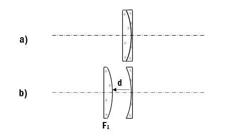
Figure 1: Variable power by varying the separation of the lens components
Now suppose that the lenses are separated by 2.4mm as shown in figure 1b, the power of the system measured at the concave surface of the -20.00 D component is given by
F1 / (1 - dF1) + F2 = 20 / (1 - 0.0024x20) - 20.00 = +1.00D
Shifting the +20.00 D lens forwards by a further 2.15mm produces +2.00 D and a shift of 10mm from the zero position produces a power of +5.00 D. Clearly, such a combination of lenses can be used to obtain a variable power system.
The change in effective power measured at the concave surface is
F1 / (1 - dF1) - F1 = dF12 / (1 - dF1)
Since d is small when expressed in metres, the denominator is not very different from unity, and the change in power, A, can be expressed as
A = dF12 / 1000
where d is expressed in millimetres. Since the numerator of this expression is always positive, it does not matter whether the front moveable lens is the plus component or the minus component.
To produce an adaptive optical system which will provide variable power from +5.00 D to -5.00 D, a -25.00 D rear component might be chosen and a +20.00 D front, moveable component as shown in figure 2. When the lenses are in contact the power of the combination is -5.00 D. If the front lens is then moved forward by 2.4mm, the power of the combination becomes -4.00 D.
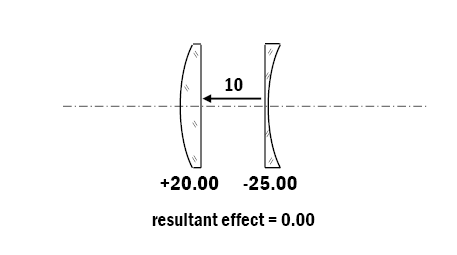
Figure 2: Variable power system designed to produce range +5.00 to -5.00 D
The components have been reversed from those shown in figure 1 in order to provide a better optical performance over a wider field with fewer off-axis aberrations, so the front surface of the plus lens must be compensated for the lens thicknesses.
In order to produce a variable power, ready-to-wear spectacle lens designed for reading purposes only, whose power covered the full permissible range suggested in BS EN ISO 14139 – Ophthalmic Optics – Specifications for ready-to-wear spectacles, of +1.00 D to +3.50 D, a back element of -19.00 D could be combined with a front moveable lens of power +20.00. Then, when the lenses are in contact they will provide a power of +1.00 D and the movement required to obtain a lens of power +3.50 D would be just 5.55mm. Requiring such a small movement of the components, a device of this nature would be very simple to construct with the front lens mounted in, say, a screw threaded cap which would not have an unusual appearance or be too cumbersome. Bennett has recorded that adaptive spectacles of this nature were patented by H Dixon3 of London as long ago as 1785.
Adaptive prism systems are well known in the form of the rotary prism. Such a device employing two 15Δ components can produce any resultant prism power from zero to 30Δ by rotating the two prisms in relation to one another. The rotary prism not only forms a useful trial case accessory, but is also used as a prism compensator in the focimeter, either to extend the measuring range of the instrument or to neutralise prism in a lens before power readings are taken.
The Stokes’ lens
Another accessory which may be found in the trial case is the Stokes’ lens which is an adaptive cylinder that can produce any cylinder power from zero up to twice the value of either component. However, the Stokes’ lens also has a residual spherical power which is always half the value of the resultant cylinder power.
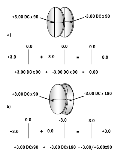
Figure 3: Stokes’ lens made with ±6.00 D Cyls in minimum and maximum configurations
Consider the pair of ±3.00 D plano-cylinders illustrated in figure 3. When placed together as shown in figure 3a they neutralise one another and the resultant effect is zero. This effect is confirmed by the optical cross representations of the principal powers shown in the figure, and the fact that they neutralise along every meridian is obvious since the absence of material from the convex cylinder is replaced by the presence of material from the concave cylinder.
If the -3.00 DC component is now rotated through 90° as shown in figure 3b, the combination becomes -3.00 DC x 180/+3.00 DC x 90 which is equivalent to -3.00 DS/+6.00 DC x 90.
Suppose now that the -3.00 DC x 90 shown in figure 3a was rotated through 30° from the zero position. The resultant, found by summing the obliquely crossed cylinders, +3.00 DC x 90/-3.00 DC x 60, is found to be -1.50 DS/+3.00 DC x 120.
This result can be found as follows. If we have two equal but opposite powered cylinders, F1 DC / -F1 DC with an angle α between their axes, we find from the theory underpinning Stoke’s construction that the axis of the resultant cylinder lies at α/2 from either axis ie, midway between their two plus axis meridians, and that the power of the resultant cylinder is given by
C = √(F12 + F22 + 2F1F2 cos 2α)
= √(2F12 - 2F12 cos 2α)
= √(4F12 sin2 α)
= 2 F1 sin α
and S = (F1 + F2 - C) / 2 = - C / 2 = - F1 sin α
For the example shown in figure 4, +3.00 DC x 90/-3.00 DC x 60, α = 30°
C = 2 F1 sin α = 6 sin 30 = +3.00 DC
S = - F1 sin α = -3 sin 30 = -1.50 DS
So the resultant is -1.50/+3.00 x 120.
If the minus cylinder is rotated through 60° from the zero position, the two components now being
+3.00 DC x 90/-3.00 DC x 30 the angle between the axis meridians, α, = 60°.
C = 2 F1 sin α = 6 sin 60 = +5.20 DC
S = - F1 sin α = -3 sin 60 = -2.60 DS
(ie half the value of the resultant cylinder)
and the combination is equivalent to -2.60/+5.20 x 105.

Figure 4: Stokes’ lens with acute angle of 30° between the axes; +6.00 DC x 90/-6.00 DC x 60
If it is required to produce variable cylinder power but to maintain a fixed axis direction, then the components must be arranged to rotate through equal angles, one clockwise and the other, anti-clockwise from the zero position, and this must lie at 45° to the required axis direction. For example, if it is required to maintain an axis direction of 45° then the cylinders shown in figure 3a would be orientated so that their common axis meridian for the zero position lay along 180 and, using the same mechanism as that found in the rotary prism, when one cylinder is rotated anti-clockwise, through 15°, so that its axis lay along 15°, the other cylinder would rotate clockwise through 15°, so that its axis lay along 165°.
The Stokes’ lens is used in some automatic refractometers when it is usually combined with an adaptive spherical lens to neutralise the spherical component which results from the variable cylinder.
Alvarez-Lohmann lenses
An adaptive lens which can provide both variable spherical and cylindrical power was described by Luis W Alvarez4 in 1967. Three years later an adaptive lens of similar construction was described by A Lohmann5 and lenses of this type are often referred to as Alvarez-Lohmann lenses. Here, for brevity, they will be called simply, Alvarez lenses.
Consider the parallel-sided block of optical material, say a block of CR 39, illustrated in figure 5a. Clearly, there would be no movement of objects viewed through the block depicted in figure 5a, under the transverse test. On careful inspection of the block it is seen that the block is actually made from two separate components which have been put together as shown in figure 5b.
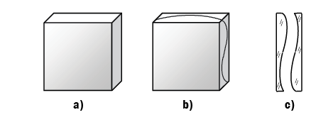
Figure 5: Components of the Alvarez lens
a) block of optical material, e.g. CR39
b) block sliced into two as indicated
c) cross-section of the two components
A cross sectional view of the two separated components is shown in figure 5c. Like the plano-convex and plano-concave cylinders which make up the Stokes’ lens, the absence of material from one component is entirely replaced by the presence of material from the second component.
Figure 6a shows that provided that the two components are sufficiently thin, despite its peculiar shape, the Alvarez lens would still be afocal if its two components were placed together, with their plane surfaces in contact. Once again, the absence of material from one component is precisely compensated for by the presence of material from the second.
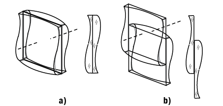
Figure 6: Alvarez lens arranged to form a positive lens
a) components in afocal position
b) components slid apart to form a plus lens
Now consider the cross-sectional shapes of the resulting element when the two components are separated by sliding the two components along their plane surfaces, as shown in figure 6b. In the figure, the components have been separated by sliding the second component downwards in relation to the first, the plane surfaces remaining in contact. It can be seen that an optical element is formed which has two convex surfaces and, it will be seen, that the thickness of this element varies in every meridian in exactly the same way as the thickness of a bi-convex spherical lens.
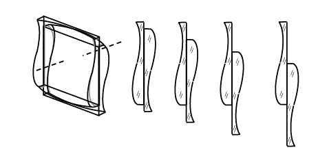
Figure 7: Increasing the separation of the elements increases the power of an Alvarez lens
Furthermore, as can be deduced from figure 7, the greater the separation of the components, the greater becomes the thickness difference across the components so the greater becomes the power of the resulting spherical lens.
In figure 8, the two components of the Alvarez lens have been slid in the opposite direction, when the resulting optical element is seen to possess two concave surfaces forming a negative lens. Once again, the further the movement of one component in relation to the other, the greater the increase in the minus power of the lens.

Figure 8: Alvarez lens arranged to form a negative lens
a) components in afocal position
b) components slid apart to form a minus lens
Now consider how the thickness of the Alvarez lens changes when, starting from the afocal position of the elements, the components are slid horizontally in relation to one another (figure 9).
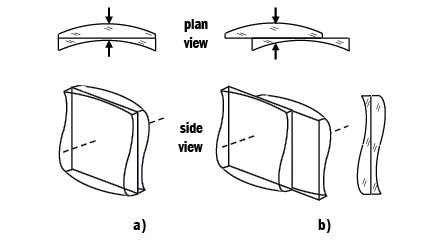
Figure 9: Alvarez lens arranged to form a plano-cylinder
a) components in afocal position
b) components slid apart to form a plano-cylinder
It can be seen that along the vertical meridian of the combination the thickness does not change, the Alvarez lens remains afocal in the vertical meridian. Along the horizontal meridian, however, as the separation increases from the zero position shown in figure 9a, the thickness of the combination starts to increase. It will be seen that this movement produces a plano-cylinder with its axis at 45°. The Alvarez lens now behaves like a plano-cylinder whose cylindrical effect increases as the separation of the components is increased along the horizontal meridian.
It follows that if the two components are separated in both the vertical and horizontal meridians the resulting Alvarez lens will possess both spherical and cylindrical power, ie, it has become a variable power sphero-cylindrical lens. As stated above, the axis of the cylinder will lie along the 45° meridian of the elements shown in figures 6 to 9.
The contact surface between the two elements does not need to be a plane surface as can be seen in figure 10 which shows a cross-sectional view of a curved form of Alvarez lens. However, in designing a curved interface, sufficient space must be allowed between the two sliding components to enable them to slide without making contact with one another.
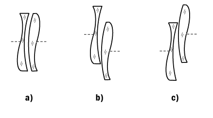
Figure 10: Alvarez lens with a curved contact surface
a) elements in afocal position
b) arrangement for plus lens
c) arrangement for minus lens
Variable power from fluid-filled lenses
If a hollow, parallel-sided, plate of glass with very thin, flexible walls is attached to a reservoir containing some transparent liquid, when the space between the walls is just filled with the liquid the filled plate will act like a parallel-sided plate of glass with no power, as illustrated in figure 11a.

Figure 11: Fluid-filled adaptive lens
a) chamber filled with fluid
b) pressure forces fluid into the chamber to produce lens
When a further volume of liquid is forced into the plate, the flexible walls will bulge outwards under the pressure of the liquid to form a bi-convex lens. Assuming the walls of the deformable plate to be thin and remain parallel-sided, they play no part in the power of the resulting lens which is due entirely to the shape of the liquid lens of refractive index, n.
On the other hand, if fluid is withdrawn from the sealed chamber it will suck the thin walls towards one another to produce a bi-concave lens as illustrated in figure 12.
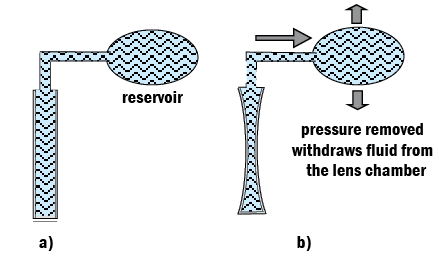
Figure 12: Fluid-filled minus adaptive lens
a) chamber filled with fluid
b) pressure removed draws fluid out of chamber to produce a bi-concave lens
The power of the resulting lens will depend upon the change in volume of the liquid. Since there is greater pressure exerted at the centre of the bi-convex lens where the thickness of fluid is greatest, the form of the convex surfaces will be paraboloidal. In the case of the withdrawal of fluid to produce a minus lens, once more, the change in thickness of the fluid will produce a pair of concave paraboloidal surfaces.

Figure 13: Volume of a paraboloidal cap
Consider the paraboloidal cap illustrated in figure 13, whose radius at the vertex is r0, and whose sag at the diameter, 2y, is z. The volume, V, of the paraboloidal cap is given by π z2 r0 and since for a paraboloid, z = y2 / 2r0 = d2 / 8r0 where, d = 2y, on substituting 100(n - 1)/F for r0, the volume of the cap is given by π d4F / 6400(n - 1) cm3, (d in cm).
The relationship between the power, F, and the volume of the lens, V, is therefore,
F = 6400(n - 1) V / π d4, V being expressed in cm3.
Suppose that the fluid contained between the walls is an oil of refractive index 1.586, and that the fluid lens is circular of diameter 42mm, ie 4.2cm. When the cavity contained by the hollow parallel-sided walls, tE, is 3mm thick, as shown in figure 13a, the volume of the cylindrical plate formed by the oil is simply
V0 = π d2 tE / 4 cm3 = π x 4.22 x 0.3 / 4 = 4.156 cm3.
In order to induce a change in power of +1.00 D, the volume of the plate must be increased by, V,
= π d4 / 6400 (n - 1) cm3 = π 4.24 / 6400 (0.586) = 0.261cm3,
when its total volume becomes V + V0 = 4.156 + 0.261 = 4.417 cm3.
The power of the lens, F, can then be expressed as
F = 6400(n - 1)(V - V0) / π d4
It can be seen from this expression that the power increases linearly with the volume of the lens.
The graph in figure 14 shows a plot of the necessary change in volume against the power of the lens. In real terms, the amount of fluid which has to be injected to increase the power of the lens by +1.00 D, or to remove from the lens to obtain a change of -1.00 D, is just a little over 0.25cm3.
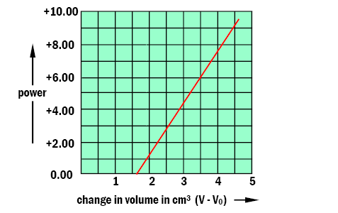
Figure 14: Graph to show the relationship between the power and the volume of a lens
Bennett records that the first known deformable lens produced by inducing a change in the power of a lens by changing its volume, was thought to have been used as an objective for a long-focus telescope, made in 1747 by a Dresden instrument maker named Grummert. A patent was granted to the French ophthalmologist Dr Cusco6 for the use of such a lens in a binocular optometer, used to study accommodation. The detail of one of his lenses is shown in figure 15 where it can be seen that one surface of the lens is rigid, only the right-hand surface being deformed when liquid is pumped into the system. The power of the variable focus lenses could be controlled to 0.01 D by an elaborate hydraulic system.
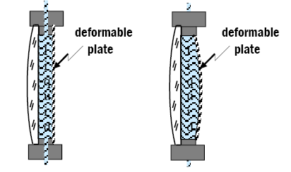
Figure 15: Dr Cusco’s deformable lens
The chief problem in designing a deformable lens is that of ensuring that the hydraulic system forms a liquid-tight cavity. A suggestion made by Dr BM Wright7 was to employ a triple-layer construction the three components being laminated together to form the lens. The front component is a glass (or plastics) lens made to the distance prescription, with any astigmatic correction on the convex surface of this component. The central layer is a circular sheet of polyvinyl butyral, 0.37mm thick, with a central circular hole some 25mm in diameter to serve as the liquid chamber. The rear component is a cover slip of glass, 0.15mm thick, capable of flexing to the extent required under pressure (figure 16).
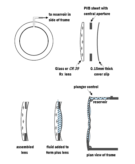
Figure 16: Dr Wright’s deformable lens
A duct 0.75mm in diameter was drilled downwards through the upper edge of the lens, opening into the liquid chamber via a short horizontally drilled hole. The fluid supply is kept in a reservoir in one of the sides and supplied to each lens cavity via a duct in each frame rim, linked via the bridge of the frame. Sliding a plunger on the reservoir side of the frame forces more fluid to enter the cavities, causing the cover slip to flex into a convex cross-section.
Sliding the plunger on the side of the frame in the opposite direction withdraws fluid from the lenses the cover slip resuming its unstressed form and the lens power to reduce.
The search for a method of providing a fluid-tight seal which could withstand the pressure from the liquid passing through such narrow ducts was unsuccessful and the design was eventually abandoned.
Although Dr Wright’s deformable lens did not reach the marketplace, the idea was revived, at the end of the 20th century in improved form by Dr JD Silver.8,9 with the introduction of his Adspec deformable spectacles. Unlike Dr Wright’s spectacles, each lens is capable of being deformed separately allowing for different spherical prescriptions to be obtained in each lens. The range of powers which can be obtained for each lens is from +6.00 to -6.00 D and successful field trials were undertaken in developing countries, which had little or no optometric facilities. It was envisaged that the cost of manufacture of these spectacles could be made sufficiently low to allow widespread distribution in countries where most people could not otherwise afford optometric correction.
The lens form employed in Dr Silver’s Adspecs is illustrated in figure 17. The fluid used is an oil of refractive index 1.579 which is contained between two very thin membranes of Mylar type ‘D’ PET film, whose refractive index varies between 1.64 and 1.67. The film is some 23μm thick, and the membranes are sealed at a diameter of 42mm. The sealed membrane is sandwiched between two flat polycarbonate plates to prevent damage to the membrane. The fluid is supplied in two cylinders attached to the sides of the frame which can be removed, once the lens powers have been selected for each eye separately.

Figure 17: Dr Silver’s adaptive spectacle lens
The range of powers covered by the Adspecs is from +6.00 D to -6.00 D, the volume change required to provide this 12.00 D power range being
12 π d 4 / 6400 (n - 1) = 3.17cm3.
This change requires the volume of the fluid contained within the sealed membranes to be increased by 1.58 cm3 to reach +6.00 D and decreased by 1.58cm3 to obtain -6.00 D.
Figure 18: Adlens Hemisphere Variable Focus Eyeglasses
The advice provided for setting the power to obtain best vision for each eye separately, is to first set the lens power to +6.00 D and then to withdraw fluid slowly while viewing a sight-test chart, until best vision is obtained to ensure that accommodation remains unstimulated. Fluid adaptive spectacles are now available from several sources such as the Adlens Hemisphere Variable Focus Eyeglasses10 illustrated in Figure 18.
References
- Bennett AG. (1972). Variable and progressive power lenses. Manufacturing Optics International, IPC Science & Technology Press, Guildford.
- Jalie M. (2016). Progressive power lenses (Part Two), Optician Vol. 252, No 6,569 p24-31.
- Brit. Patent 1515 (1785) Dixon H. Telescopes, microscopes spectacles, etc.
- US Patent 3305294 (1967) Alvarez LW, Two-Element Variable-Power Spherical lens.
- Lohmann, A. (1970) A new class of varifocal lenses. Applied optics 9, 1669–71 (1970).
- Fr. Patent 129293 (1879), Dr Cusco, Système de lentille à foyer variable sans déplacement.
- Demonstrated at the Physical Society’s Exhibition in 1968.
- Afenyo, GD and Silver, JD. (2001) Vision correction with Adaptive Spectacles World Blindness and its Prevention, Vol. 6. International Agency for the Prevention of Blindness, Hyderabad, India.
- Douali, MG and Silver, JD. (2004) Self-optimised vision correction with adaptive spectacle lenses in developing countries. Ophthal Physiol Opt. 2004 24: No. 3
- www.adlens.com