Artificial intelligence (AI) is increasingly being used to develop automatic systems for medical image analysis. In the field of eye care there have been significant efforts to develop systems that automatically detect age-related macular degeneration (AMD) in optical coherence tomography (OCT) and fundus photographs with the aim to support eye healthcare services in disease diagnosis and monitoring.1,2 Neural networks form the base of deep learning and represent a subfield of AI where it is often discussed that neural networks require large amounts of data to learn. But how do they learn and why is big data important? The aim of this article is to answer these questions by introducing how convolutional neural networks (CNN), a fundamental class of deep learning neural network most commonly used for image classification, work through the example of addressing a major challenge for primary care providers – the detection of early features of AMD.
The problem space
When AMD is diagnosed in the early non-exudative stage (dry AMD) patients can begin sight preserving lifestyle changes. An early defining feature of dry AMD is abnormal accumulation of macular drusen. However, as drusen occurs asymptomatically in normal aging it is challenging to discern between potential early pathological features of AMD and age-related drusen. Early AMD is more often identified in the later stages either incidentally at a routine eye exam or when an individual is symptomatic with potential sight threatening late AMD (wet AMD). Drusen is time-consuming and challenging to manually detect and quantify where an automatic method would significantly alleviate the task. Therefore, developing tools to automatically quantify drusen (eg count, size, location) would help an optometrist to monitor drusen for risk of conversion to wet AMD in primary care. Furthermore, if OCT is unavailable, developing automatic drusen quantification in colour fundus photographs would provide support for practices with limited resources.
To the human eye, drusen appear as bright white or yellow spots on a colour fundus photograph, but to a computer, the input image is an array of numbers (pixel values) and the size of the array is the size of the image. For example, a colour fundus photograph has three channels (red (R), green (G), blue (B)) with a size of 909 x 909 pixels where a drusen pixel would look yellow/orange/white to a human. However, to a computer, this would be (255, 219, 88). The three values correspond to the pixel values in each of the RGB channels that gives the orange colour of the retina we see on the computer screen. The aim of a CNN is to process these pixel values to learn what is in the image (such as colours, edges, shapes, textures and objects) to output a probability that the image belongs to a certain class. In this example, the aim is to classify small crops from an image (called patches) as ‘drusen’ or ‘no drusen’ (ie background, vessels, optic disc with no drusen present).
First, we must obtain some training data to train the network and testing data to see how it performs compared to a human (figure 1). Let us say we have collected thousands of colour fundus photographs featuring early AMD and visually healthy individuals over the age of 50. First, we use a grid to divide the image into small patches (figure 1B). Next, the patches are labelled by a human as drusen and no drusen by assigning a value of 1 or 0, respectively (figure 1C). Then, we subset 70% of the images (and their corresponding labels) to make our training set (figure 1D). The remaining 30% of the images (and their corresponding labels) make up the independent testing set (figure 1E). Finally, the aim is to apply the trained network to each grid cell in the testing set to automatically classify whether it contains drusen or no drusen. Since we have manual labels in the testing set, we can compare the trained CNN’s predictions to the manual annotations to assess its performance. Using this design, we can also automatically quantify drusen location (using the grid cell locations) and counts (by counting how many grid cells were classified as drusen) to investigate the associations between age-related drusen and early AMD or to propose a tool to monitor AMD progression.
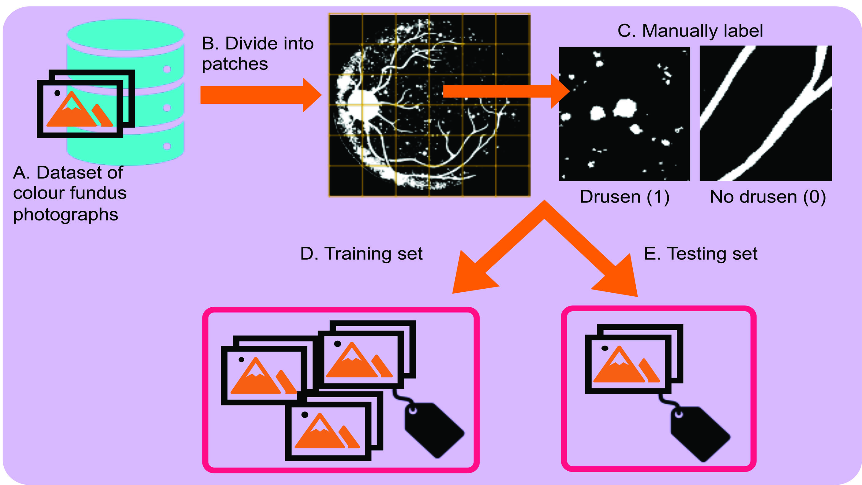 Figure 1: Obtaining training and testing data for the task of drusen detection
Building a CNN
The artificial neuron
The building block of a CNN is an artificial neuron that is inspired by the human neuronal cell. Just as a biological neuron receives signals from synaptic junctions and processes the signal in the cell body to output a response, so too does an artificial neuron.
Figure 2 shows the artificial neuron and its conceptual derivation from biology. A neuron accepts multiple inputs, called weights (w) and performs a mathematical operation to output a ‘response’. The operation consists of summing all input weights (the dot product) and adding a bias value (b). The bias value is constant and is required to prevent the sum of the input equalling 0 (otherwise there would be no output). The output from the neuron is called an activation function (ƒ). Many activation function formulas exist, where the primary aim of an activation function is to normalise outputs to a certain numeric range to prevent the output having an infinite value. Popular activation functions include the sigmoid function that scales the values between 0 and 1.
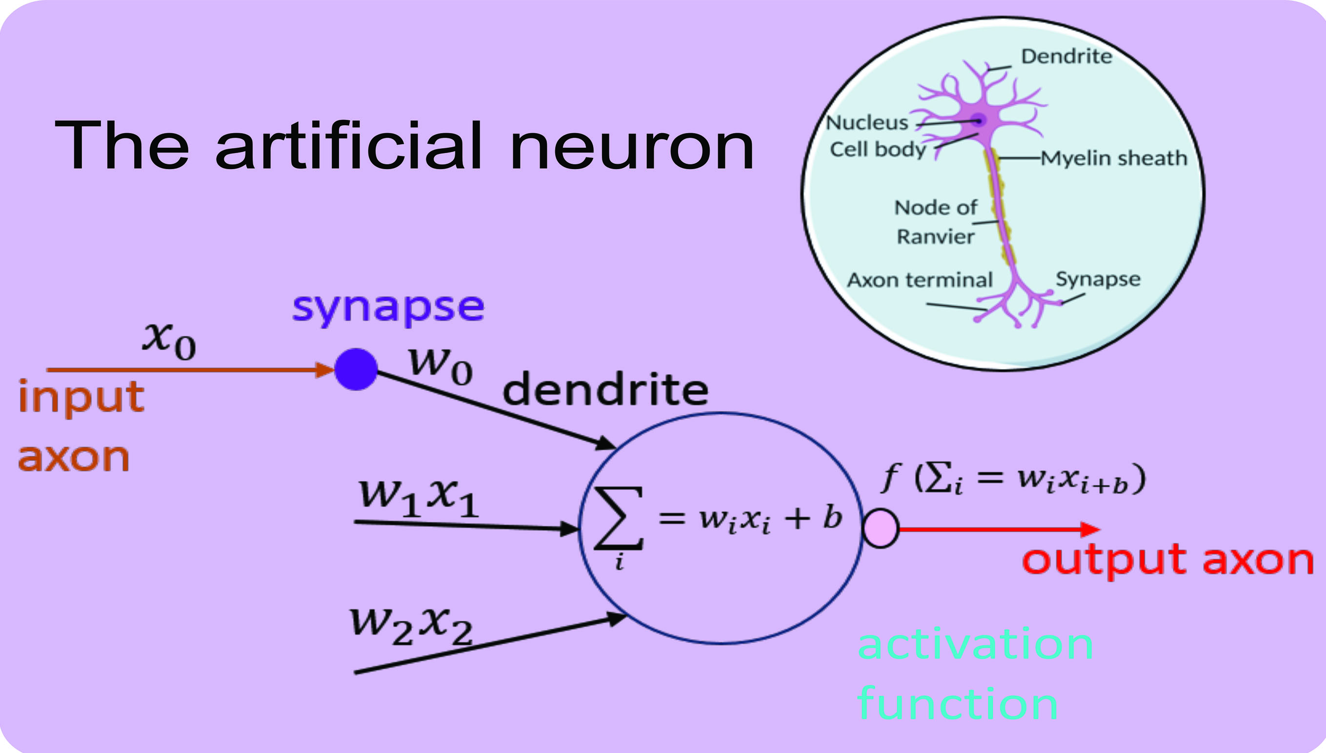 Figure 2: The artificial neuron and it’s biological derivative3
Pioneering studies by Hubel and Wiesel revealed that cells in the visual cortex of the brain are organised in layers that respond and filter different sensory information in order to output a response.4 A deep learning neural network is inspired by this structure, where neurons are also organised into layers where each neuron in a layer accepts inputs from the previous layer, performs an operation and outputs a response that is passed to the next layer, and so on. All the layers of a neural network therefore consist of multiple neurons that receive their weights from the input image or from the neurons in the previous layer. The intuition behind a CNN can be thought of as (1) feature extraction, whereby descriptions of what is contained in the image (eg blood vessels) are detected and is achieved by layers called convolution and pooling and (2) classification, whereby the features are used to assign a probability to the input that it belongs to a certain class and is achieved by a fully connected (FC) layer.
Convolution
The first layer of a CNN is called convolution and works by comparing an image piece by piece (called a filter) and gives the neuron its initial input weight. Convolution is often described as shining a spotlight of a certain size over the input image where the values in the filter are compared to the area on the image that is illuminated to output a weight.
Figure 3 shows, as an example, convolution applied to a ‘drusen patch’ where we have already learned the values of the filters (ie the features). In this example, the filter we are applying is a 3x3 array with values of -1 for black and 1 for white and pertains to an already learned feature of an edge-like object (figure 3A). Next, the filter is applied to each position on the input image (or convolved) (figure 3B). The pixel value in the filter is multiplied by the corresponding pixel value in the input image, summed and divided by the size of the filter (3x3 = 9) (figure 3C). The output of each position of the filter (ie a neuron weight) is stored as an activation map, where values close to 1 correspond to close matches to the filter, a value close to -1 is a strong match for the photonegative of the image and values close to 0 are no match. (figure 3D). In this example, the edge filter detects features with similar shape and can be seen in the activation map (ie the neurons have ‘fired’). The values of the filters (ie the features) are learned during training. 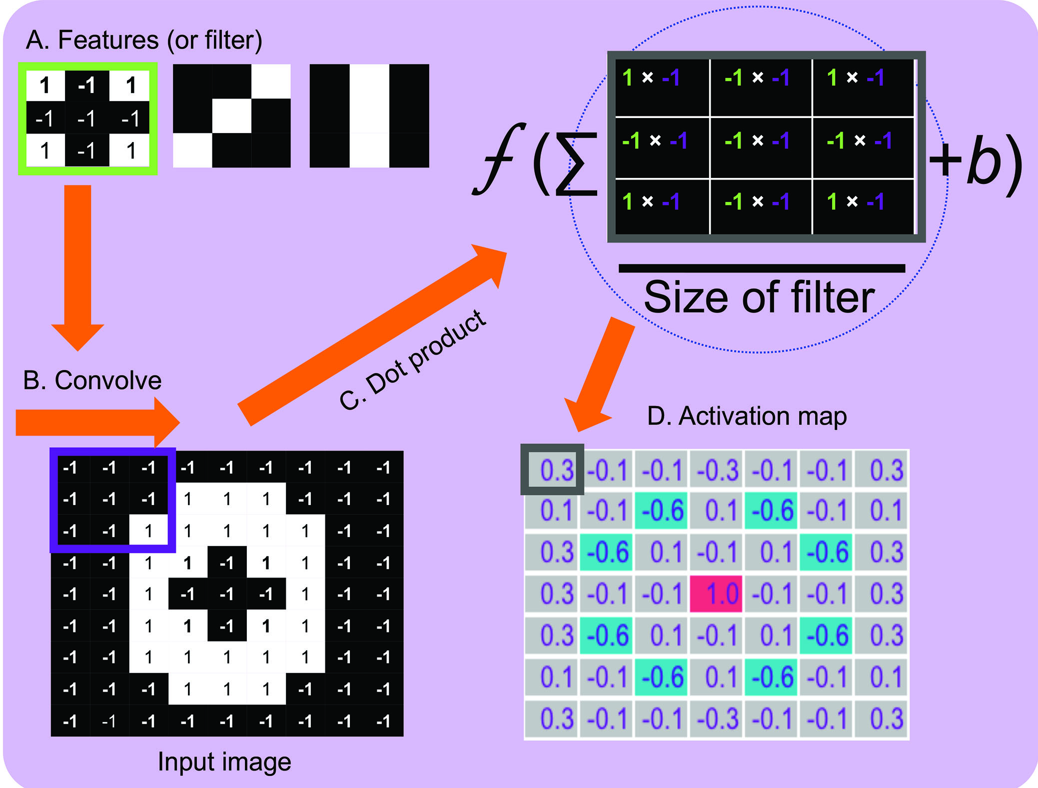 Figure 3: Convolution applied to a ‘drusen’ image patch. The values in the activation map are the dot products prior to the application of the activation function for illustrative purposes. If we apply the sigmoid activation function to the value 0.3 the output in the activation map would be 0.54
This describes convolution in a 2D space on a small 9x9 image, but in reality, fundus photographs have three channels and are much larger (ie higher dimensional). A commonly used input size into a CNN is 224x224x3 (three for the RGB channels; ie an input volume), this is because performing convolutions on a large image will be computationally impractical. One could resize a whole fundus image and input into the network but would result in a lower image resolution and since drusen are small we may lose valuable features. For the task of drusen detection dividing the image into patches allows us to preserve details during training. As before, the filter convolves across the height and width of the input volume and computes the dot product between the values in the filter and the values in the volume from the height, width and depth dimensions (3x3x3). Effectively, for every position of the filter on the input image there is a single neuron and for every filter there is a 2D activation map that is then stacked to give an output volume. This is how CNNs capture information from all three channels of an input image and detect features (figure 4). 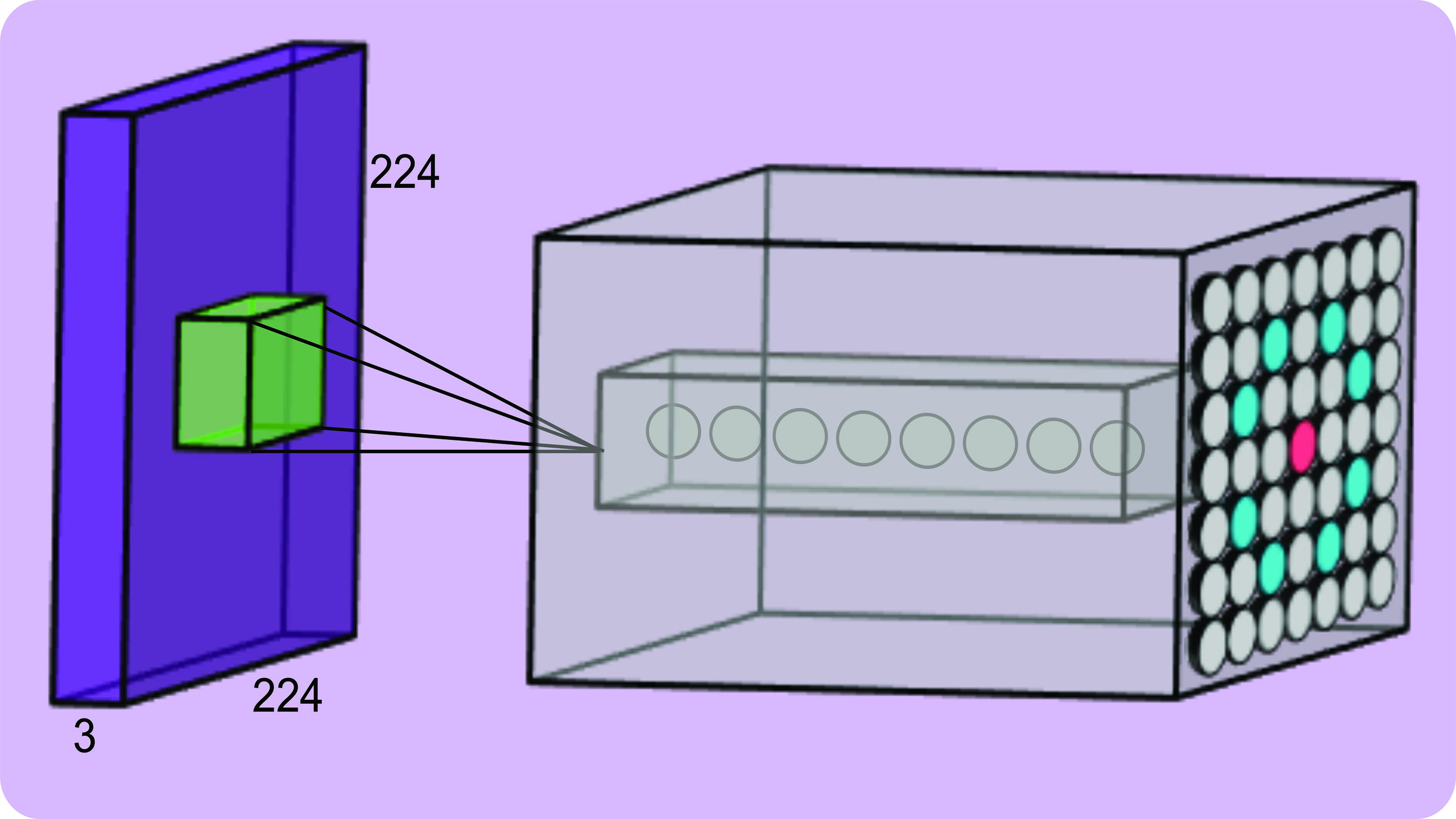 Figure 4: An input volume (purple) with an example output volume (grey)
Pooling
The aim of our CNN is to output a single value (ie probability) that an image belongs to a certain class (eg drusen or no drusen). To progressively reduce the input image and its output volume to a single probability value different types of layers are inserted into the neural network architecture. For example, pooling is applied whereby a window of a specific size is walked along the output of the previous layer (much like convolution) and the average value (so called average pooling) or the largest value (so called max pooling) is extracted from each activation map that returns a stack of smaller activation maps. The architecture of a simple CNN consists of repeating combinations of convolution and pooling layers that results in an output that is smaller and smaller in each layer. Each layer captures different levels of details, where in early layers simple features in the image, such as edges, are captured and in later layers high-level features are captured, such as the structure of blood vessels. This is because as the activation maps are progressively convolved to smaller activation maps more detail is present in the earlier layers and become more abstract or coarse in the later layers (figure 5).
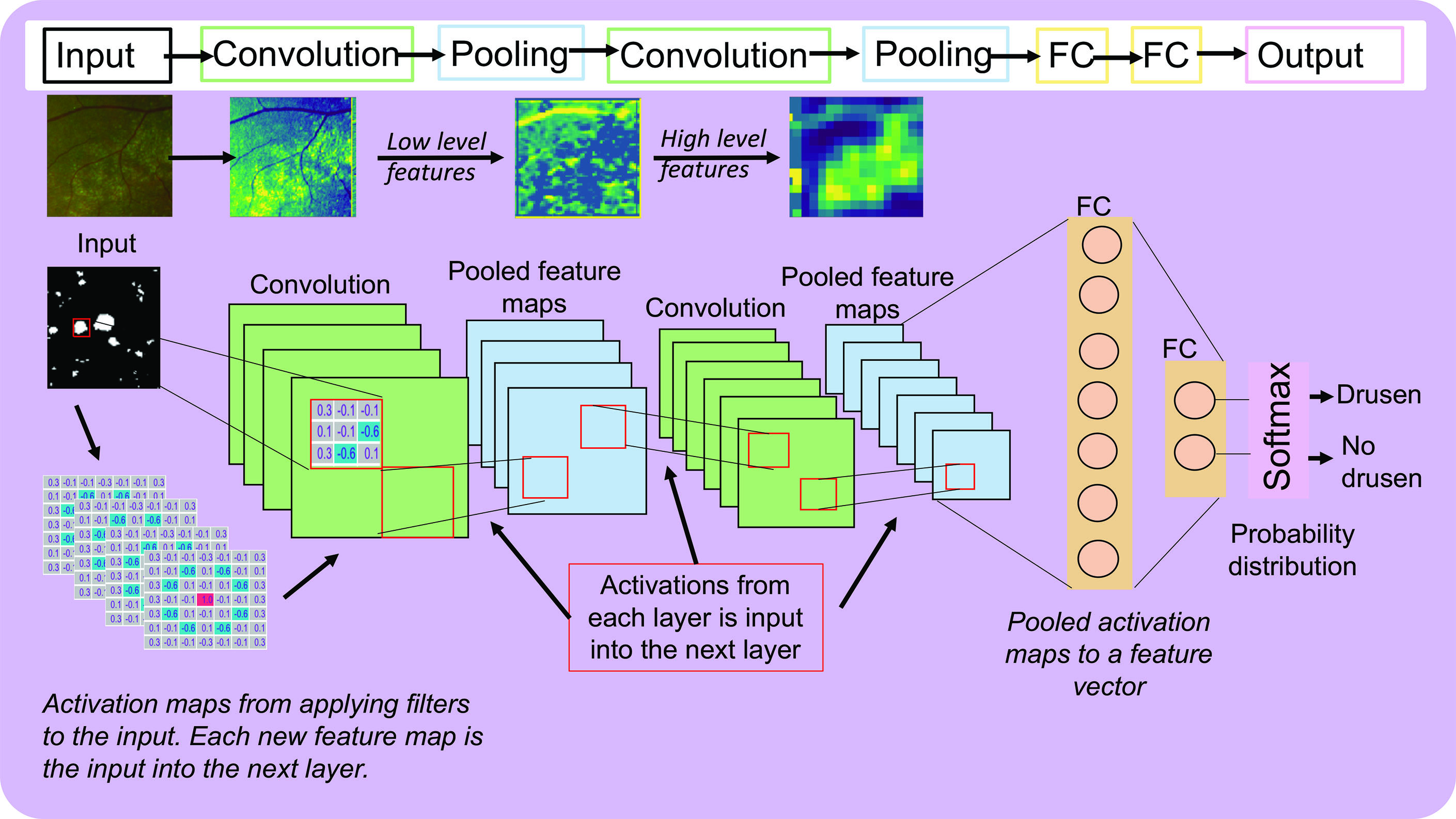 Figure 5: A simple CNN architecture and an example of activation maps from a CNN previously trained on patches of drusen and no drusen from UWF fundus images3
Fully connected layer
The final layer of a neural network is FC layer that takes the output of the previous later (eg convolution or pooling), flattens it, and outputs an N by 1 array, where N is the number of classes we would like to predict (eg N = 2 for classifying no drusen and drusen). This layer combines all the values of the previous layer, distributes them into a range of 0 or 1 (ie a probability distribution) using an activation function and outputs a probability of the input image belonging to a certain class. Many activations exist, but the most commonly used are called sigmoid and softmax (figure 5).
CNN architecture
Figure 5 shows the architecture of a simple CNN consisting of the all the components discussed so far. In this example, a drusen patch is passed through the first convolutional layer and filters
are applied resulting in a stack of activation maps (ie the output volume). The activations are then input into a pooling layer and results in a stack of smaller activation maps. This is repeated for another convolutional and pooling layer. To illustrate how this looks on a real image, a patch of drusen obtained from an ultra-widefield (UWF) fundus photograph is input into the CNN where in the first convolutional layers there are high activations (yellow) for the edges of drusen and pertain to low level features.3 As this image is passed through the network the activation maps become more abstract where in the final layer there are areas of high activation for high level features such as the whole cluster of drusen. In the final FC layer, there will be certain weights that will be high and would contribute to a higher probability that it belongs to the drusen class. These high values come from the high activations (or neuron ‘firing’) from certain features as seen in
figure 3.
CNN learning
When a CNN is first constructed the values of the filters, weights and biases of all the neurons in the network are randomly assigned a value and are iteratively adjusted during training. Neural network learning is achieved through a process called backpropagation and can be divided into four sub-processes: the forward pass, loss function, backward pass and weight update.
The forward pass involves feeding an image through each layer of the network where the final layer outputs a probability the input image belongs to a certain class. This is likely to be a low probability because all the values of the filters, weights and biases are random and have not learned any features. This returns an error and how it is computed is called a loss function. For example, if a drusen patch is input into the randomly initialised network the final layer may output 0.01 but we know the value should be 1, therefore the error given by the loss function will be high. During training, the loss is monitored because we expect this to decrease as the network learns (ie getting closer and closer to the correct prediction). The aim of the backward pass is to adjust all of the values of the filters, weights and biases in the network to minimise this error. This is achieved through a method called gradient descent.
Gradient descent can be thought of as backpacker on a hill whose aim is to be as close to the bottom of the hill as possible (figure 6A). The backpacker does not have a map and takes a step in a direction they think will take them lower, where they observe that they have indeed descended (figure 6B). They continue in this direction until they notice that they have started to ascend again (figure 6C). Subsequently, they return to their previous step and have now reached their target to be at the bottom of the hill (figure 6B). Just as the backpacker moves in different directions on the hill to minimise their height, so too does the loss function to the value of all the weights to minimise the error. 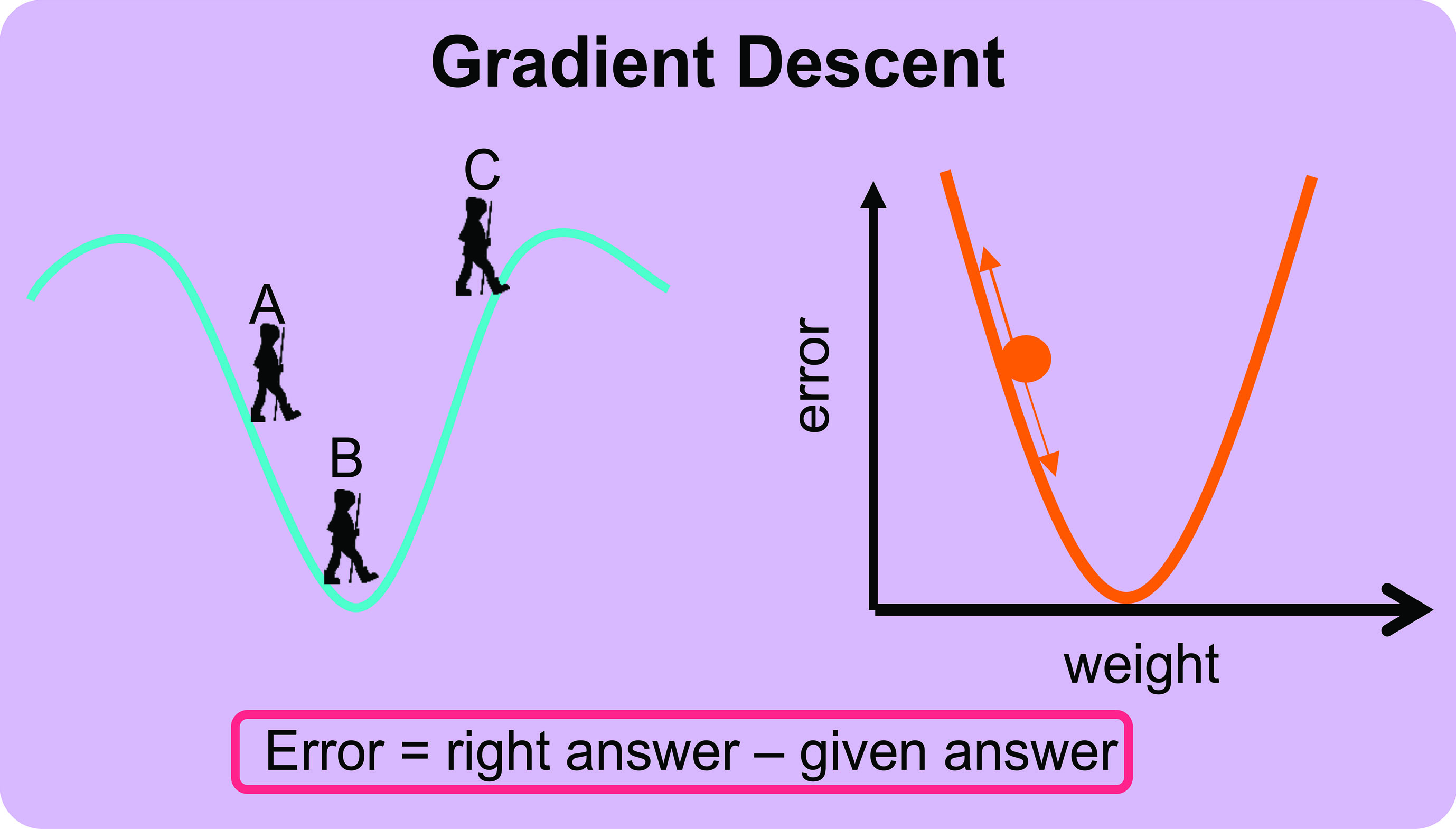 Figure 6: The concept of gradient descent3
The weights of the neurons in the neural network are therefore adjusted (the size of this adjustment is called the learning rate) to be as close to the correct answer as possible. As more and more data are fed into the network the weights, biases and outputs are continuously updated to obtain a correct prediction and patterns are eventually learned. If the neural network is trained with large amounts of data, the pattern is stabilised, and the network achieves good performance on independent testing sets.
Testing
Training a CNN is usually considered complete when the loss no longer decreases, meaning that the values of the filters, weights and biases are considered to be at their optimum value and the error cannot be further minimised. The trained network can then be fed a dataset consisting of unseen testing set to assess its performance.
Presented here is the early work from the Scottish Collaborative Optometry-Ophthalmology Network e-research (SCONe).5 A CNN was trained in a similar fashion as discussed in this article and was applied to each grid cell in the testing image to predict drusen or no drusen (figure 7A). The output predictions of each grid cell were colour coded where red regions correspond to high probability areas of drusen and blue corresponds to low probability areas for drusen (figure 7B). The output is further divided into regions to propose a method to assess drusen load in and around the macula. 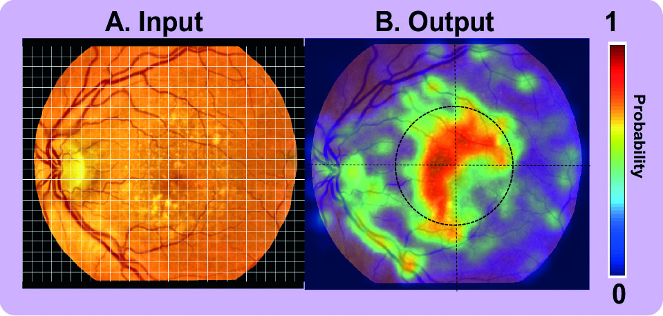 Figure 7: Example of an input colour fundus photograph with drusen5
Such a tool could support eye healthcare professionals in monitoring changes in drusen number and distribution to aid in diagnosis, triage prioritisation or for research into the pathophysiology of early AMD. Although the system seems promising, there are regions of false positives and false negatives. Sources of false positives are due to objects in the image that have a similar bright round appearance to drusen (ie similar features), whereas sources of false negatives are due to small discrete drusen that are indiscernible from the texture of the ageing retina and confounds the automatic system. For such a system to be deployed in a clinical or research environment without the need for human intervention, performance would need to be improved. This can be achieved through collection of larger training datasets as well as implementing deep learning techniques that go beyond a CNN.
Discussion
The architecture of a deep learning neural network is formed by combinations of convolutions, pooling, activations, learning parameters, loss optimisation strategies and are not limited to what is discussed here, where neural networks exist in a variety of complex and deeper architectures. In the example described here image labels are known (so called supervised learning), where there are also networks that classify images when image labels are not available (so called unsupervised learning). Unsupervised networks offer an attractive solution in the healthcare setting where obtaining large labelled datasets is challenging but evaluating such a system’s performance is no trivial matter to resolve and still requires evaluation to a reference standard. Methods have also been developed for the task of segmentation (ie classifies pixels) of drusen, exudates, microaneurysms, retinal vasculature and architecture to derive quantitative measures for risk prediction or deriving biomarkers of the body and brain.6 So called semantic segmentation requires detailed hand-drawn annotations to learn from, which is often not feasible or reliable to obtain due to time constraints, costs and inter-observer subjectivity.
It becomes clear that a deep learning system is only as good as the data it is given to learn from and obtaining large labelled datasets is challenging in a healthcare setting. Transfer learning is another method that is increasingly used for medical image analysis, whereby the weights in the early layers of a network previously trained for a different task are harnessed (ie uses previously learned features) and only the final FC layer is retrained for a new task (so-called fine tuning) and requires much smaller labelled datasets to train. However, it is unclear as to how these methods perform in a clinical environment. Additionally, systems proposed in the literature are often trained on datasets that are of high imaging quality and do not have a broad demographic range such as a range of health/disease, age, race/ethnicity and sex/gender highlighting a potential bias in AI systems.6,7 A candidate solution to this challenge is collecting the data available in high street optician practices that feature fundus and OCT images from a broad demographic range as well as linked patient data (ie already labelled images).
The future of AI in optometry is not to replace the expertise of an optometrist entirely but rather an assistive role. In the example described here, the output of a heatmap to show high probability regions of drusen could be used to visually display changes in drusen between images both to inform the healthcare provider and the patient. Especially where lifestyle changes are required, the ability to communicate to the patient through visuals may significantly improve self-management of chronic disease and help to reduce hospital referrals. Additionally, there is an increasing body of evidence that systemic (eg cardiovascular disease and chronic kidney disease) and neurogenerative diseases (eg Alzheimer’s disease) also manifest in the retina.8,9 In the future, optometrists may be able to use AI technologies to provide a variety of information about a patient’s health at a routine eye exam.
Conclusion
Through discussing how a neural network works we can understand why big and labelled data is important. In the current pandemic optometrists have had to change the way they operate, such as reservation of face-to-face assessment for essential eye care and the introduction of remote consultations, which raises the question as to how AI systems can aide eye healthcare providers in the post-coronavirus era. The answer lies within historic images and linked data from a broad demographic range that currently resides in high street practices. Such data can be used to build high performance AI tools that are assistive, such as automatic analysis of drusen to aide in screening for early AMD where there is a backlog of cases due to the coronavirus pandemic.
Dr Emma Pead is Research Fellow in Retinal Image Analysis, Centre for Clinical Brain Sciences, the University of Edinburgh.
References
- E. Pead et al., “Automated detection of age-related macular degeneration in color fundus photography: A systematic review.,” Surv. Ophthalmol., vol. 64, no. 4, pp. 498–511, Feb. 2019, doi: 10.1016/j.survophthal.2019.02.003.
- J. Yim et al., “Predicting conversion to wet age-related macular degeneration using deep learning,” Nat. Med., vol. 26, no. 6, pp. 892–899, 2020, doi: 10.1038/s41591-020-0867-7.
- E. Pead, “Assessing neurodegeneration of the retina and brain with ultra-widefield retinal imaging,” The University of Edinburgh, 2020.
- D. H. Hubel and T. N. Wiesel, “Receptive fields, binocular interaction and functional architecture in the cat’s visual cortex,” J. Physiol., vol. 160, no. 1, pp. 106–154, Jan. 1962, doi: 10.1113/jphysiol.1962.sp006837.
- E. Pead, M. O. Bernabeu, T. MacGillivray, A. Tatham, N. Strang, and B. Dhillon, “The Scottish Collaborative Optometry-Ophthalmology Network e-research (SCONe),” 2020. https://www.ed.ac.uk/clinical-sciences/ophthalmology/scone.
- M. Badar, M. Haris, and A. Fatima, “Application of deep learning for retinal image analysis: A review,” Comput. Sci. Rev., vol. 35, p. 100203, 2020, doi: https://doi.org/10.1016/j.cosrev.2019.100203.
- A. J. Larrazabal, N. Nieto, V. Peterson, D. H. Milone, and E. Ferrante, “Gender imbalance in medical imaging datasets produces biased classifiers for computer-aided diagnosis,” Proc. Natl. Acad. Sci., vol. 117, no. 23, pp. 12592 LP – 12594, Jun. 2020, doi: 10.1073/pnas.1919012117.
- M. A. Gianfrancesco, S. Tamang, J. Yazdany, and G. Schmajuk, “Potential Biases in Machine Learning Algorithms Using Electronic Health Record Data,” JAMA Intern. Med., vol. 178, no. 11, pp. 1544–1547, Nov. 2018, doi: 10.1001/jamainternmed.2018.3763.
- S. McGrory, J. R. Cameron, E. Pellegrini, and T. MacGillivray, “The application of retinal fundus camera imaging in dementia: A systematic review,” Alzheimer’s Dement., vol. 6, pp. 91–107, 2017.
- S. K. Wagner et al., “Insights into Systemic Disease through Retinal Imaging-Based Oculomics,” Transl. Vis. Sci. Technol., vol. 9, no. 2, p. 6, Feb. 2020, doi: 10.1167/tvst.9.2.6.