I first encountered optical coherence tomography (OCT) roughly 16 years ago. I had never used it before that time and had not read any material on the subject. When I saw a retinal scan, it seemed to be somehow familiar to me. I then remembered the physiological drawings from ocular anatomy books going right back to my earliest studies in 1990 with Pipe & Rapley and their anatomy book.
Since then, I have found this approach has made understanding OCT much easier – going right back to the basics. This is my aim with this series of articles (at least initially). Many clinicians and new users of OCT find much of the scans and the way they are presented difficult to understand.
Hopefully, I can help to remove some of the mystery many feel surrounds OCT.
A Basic Introduction to OCT
What is OCT? It stands for optical coherence tomography.1 Most eye care professionals have heard the term, and most know what OCT images look like. However, what is OCT for?
OCT is used to provide high-definition cross sectional images of ocular tissue and structures. Often, the technology will differentiate layers of the retina, for example, to help clinicians better understand any lesions or ocular conditions they might find.
OCT was not specifically designed for the eye. It is an imaging technique that is used in many areas of medicine, industry and technology. For example, not only is OCT used to provide images and measurements of ocular layers, but it is also used to image the inside of blood vessels, to image dental surfaces, in dermatology, gynaecology and in many other areas.2 It is also used to image materials and complex objects in very high detail in industry and science.
For the purposes of these articles, we will exclusively concentrate on ocular OCT and its many applications.
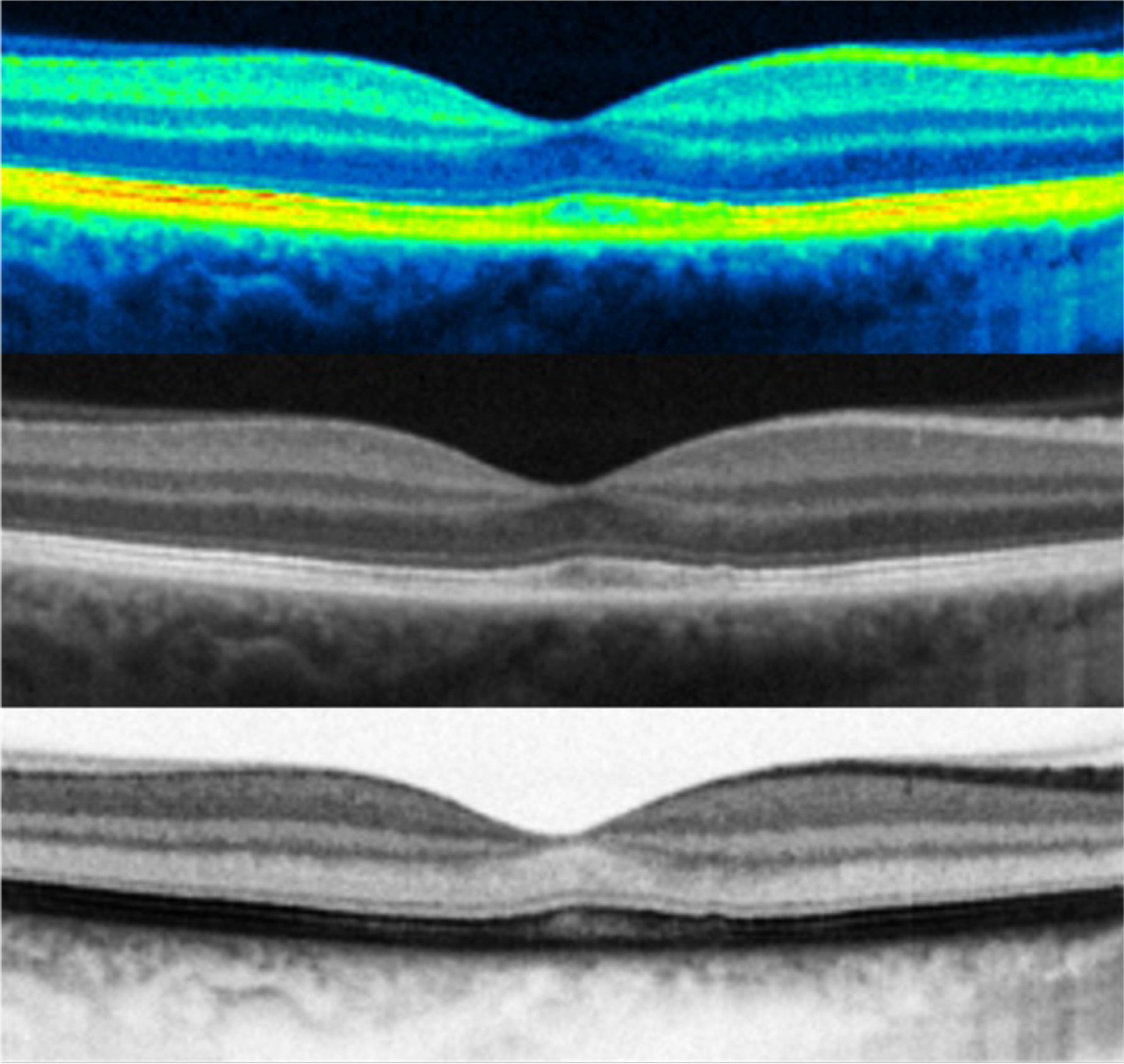
Figure 1: Examples of false colour, positive black & white and negative black & white B-Scans of the macula (same eye)
Basic Terminology
Some of the terms used in OCT come from older technology, like ocular ultrasound.
A-Scan – this is essentially the signal that enters the eye. Multiple A-Scans per second are sent into the eye in various patterns to make up varied forms of scans. Most of the modern OCT devices send between 26,000 and 400,000 A-Scans per second into the eye. The more A-Scans you can use, the more information you can obtain and, often, the higher the quality of the OCT B-Scan.3
B-Scan – this is the cross-sectional image built up from numerous A-Scans. B-Scans can be of the posterior eye (retina and optic nerve for example) or of the anterior eye (cornea, sclera and iris for example).4, 5 B-Scan images can be viewed in positive black and white, negative black and white and in false colour.
I remember looking at ocular anatomy histology slides when studying many years ago. I found, when I first saw an OCT B-Scan of the retina, it resembled the histology slides closely. This helped me to better understand the B-Scans more rapidly.6
The earliest OCTs used a beam splitter within the device to send a signal into the eye and the same signal to a reference detector. All the optical structures of the eye return some reflected signal back to the device, with subtle time differences compared to the reference.
This allowed the device to build up a picture of the various reflective and non-reflective layers using what became known as Time Domain OCT. The images were grainy and of low resolution, but, at the time, they were also a revelation. The resolution was partly determined by how many A-Scans per second could be scanned.
Later, an improved technique was developed. The software instead compared the wave composition coming back from each structure to that of the reference beam and to determine interference patterns; the result was a higher resolution image.
This type of technique became known as Fourier, or, more commonly, spectral domain (SD) OCT. In general, the signal is created by a low energy infrared laser, which scans across the entire central retinal area or a smaller region.
Latterly, newer methods of acquiring even higher resolution images have been developed. Swept source OCT rapidly sweeps between varied wavelengths of emitted laser to create a broader more detailed and complex array of interference patterns. This allows for more A-Scans per second to develop very high-resolution images.
One more very recent advancement is what is termed hyper parallel OCT, with an array of individual beamlets (rather than scanned beams). This can acquire very detailed 3D images of multiple structures and shows considerable promise in improving imaging further still.
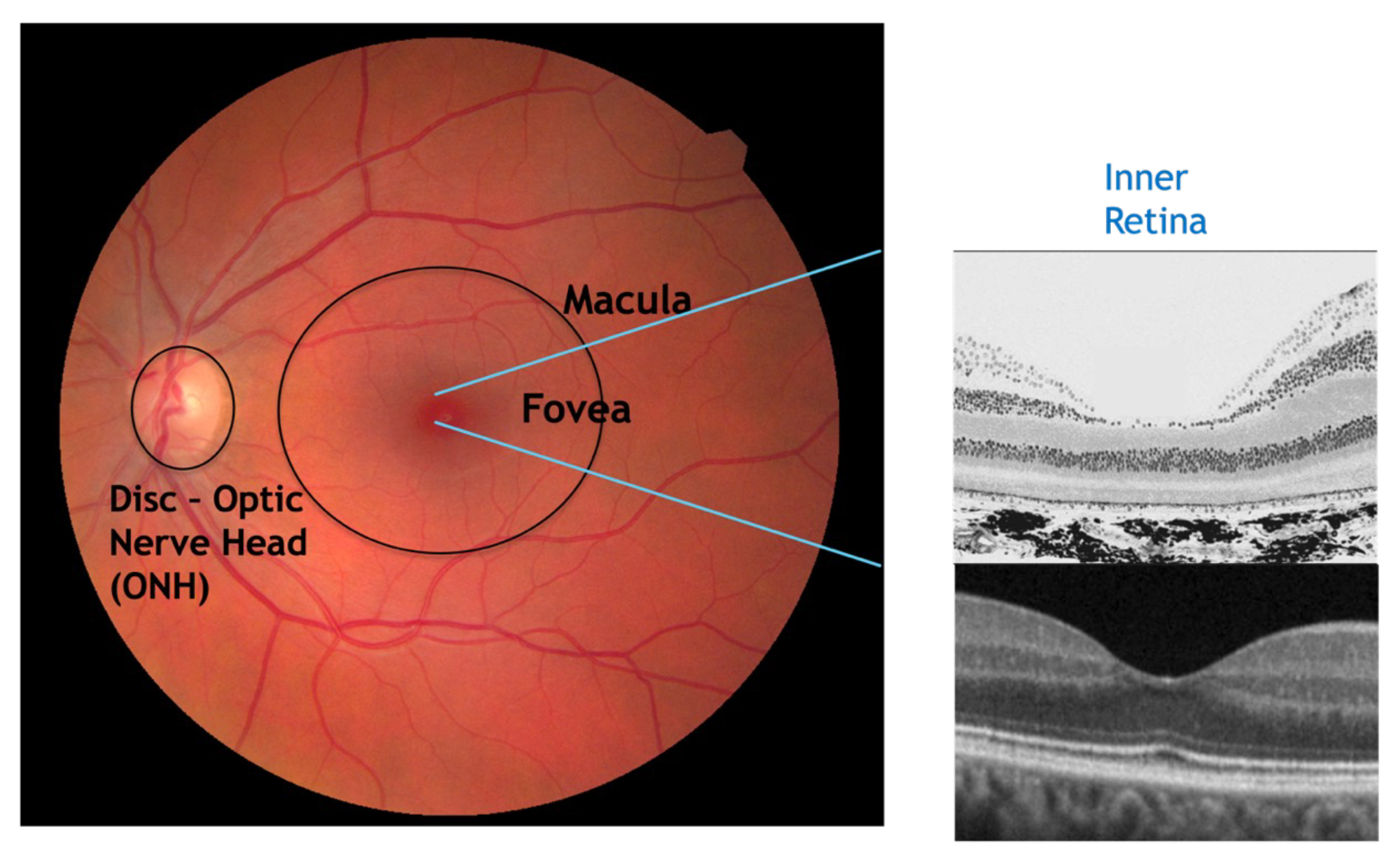
You can see in figure 2 the cross-sectional view of the central macula and fovea. You can see how the inner retinal layers are not present at the foveal pit. This is an important structure and acts as a landmark to understand the localisation of retinal lesions and their likely effect on the patient’s vision. The closer to the fovea and the foveola (central foveal pit), the more likely vision will be affected.
Figure 2: Colour fundus image and retinal histology image with OCT B-Scan
When we look at the retinal layers in some detail, there are several points I think are important to remember with regards to what should and should not be present in certain layers and what functionality certain layers have.
The retina comprises 10 distinct layers, organised from the innermost layer adjacent to the vitreous humour to the outermost layer next to the choroid. These layers, in order, are:
- Inner limiting membrane (ILM): The innermost boundary of the retina, formed by the footplates of Müller cells and in contact with the vitreous humour.
- Nerve fibre layer (NFL): Contains the axons of ganglion cells, which converge at the optic nerve head to form the optic nerve.
- Ganglion cell layer (GCL): Houses the cell bodies of ganglion cells, which are the final output neurons of the retina, transmitting visual information to the brain.
- Inner plexiform layer (IPL): A synaptic layer where bipolar cells connect with ganglion cells and amacrine cells, facilitating complex signal integration.
- Inner nuclear layer (INL): Contains the cell bodies of bipolar, horizontal and amacrine cells, which are essential for processing visual information before it is transmitted to the brain.
- Outer plexiform layer (OPL): The site of synaptic interactions between photoreceptors, bipolar cells, and horizontal cells.
- Outer nuclear layer (ONL): Contains the cell bodies of photoreceptors (rods and cones), which are responsible for detecting light and initiating the visual process.
- External limiting membrane (ELM): A thin layer formed by junctional complexes between Müller cells and photoreceptors, acting as a barrier and contributing to retinal integrity.
- Photoreceptor layer (PRL): Contains the inner and outer segments of photoreceptors, which capture light and initiate phototransduction.
- Retinal pigment epithelium (RPE): A monolayer of pigmented cells adjacent to the choroid that supports photoreceptor function by recycling visual pigments and phagocytosing shed photoreceptor outer segments.
From figure 3, we can see that the innermost five layers of the retina are the vascular retina.7 This means they have capillaries present from the retinal blood supply (via the optic nerve head). The largest capillaries are innermost (nearest the top of a B-Scan) and the smallest capillaries normally do not encroach on the outer plexiform layer. These tiniest capillaries often leak earliest in conditions like diabetic retinopathy, so micro-aneurysms and dot haemorrhages tend to appear roughly around the inner nuclear layer.8
Figure 3: Retinal anatomy with understanding of the blood supply
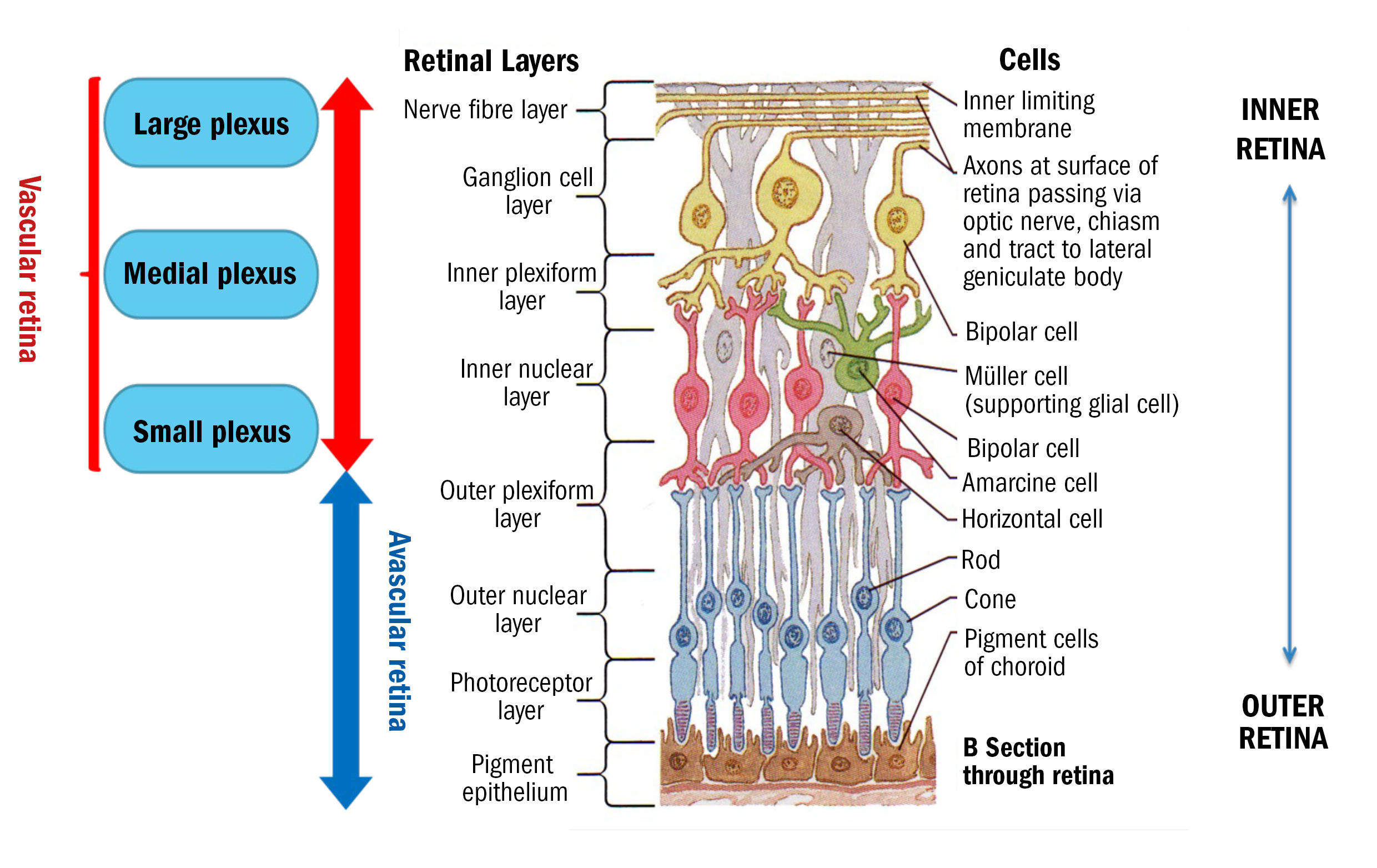
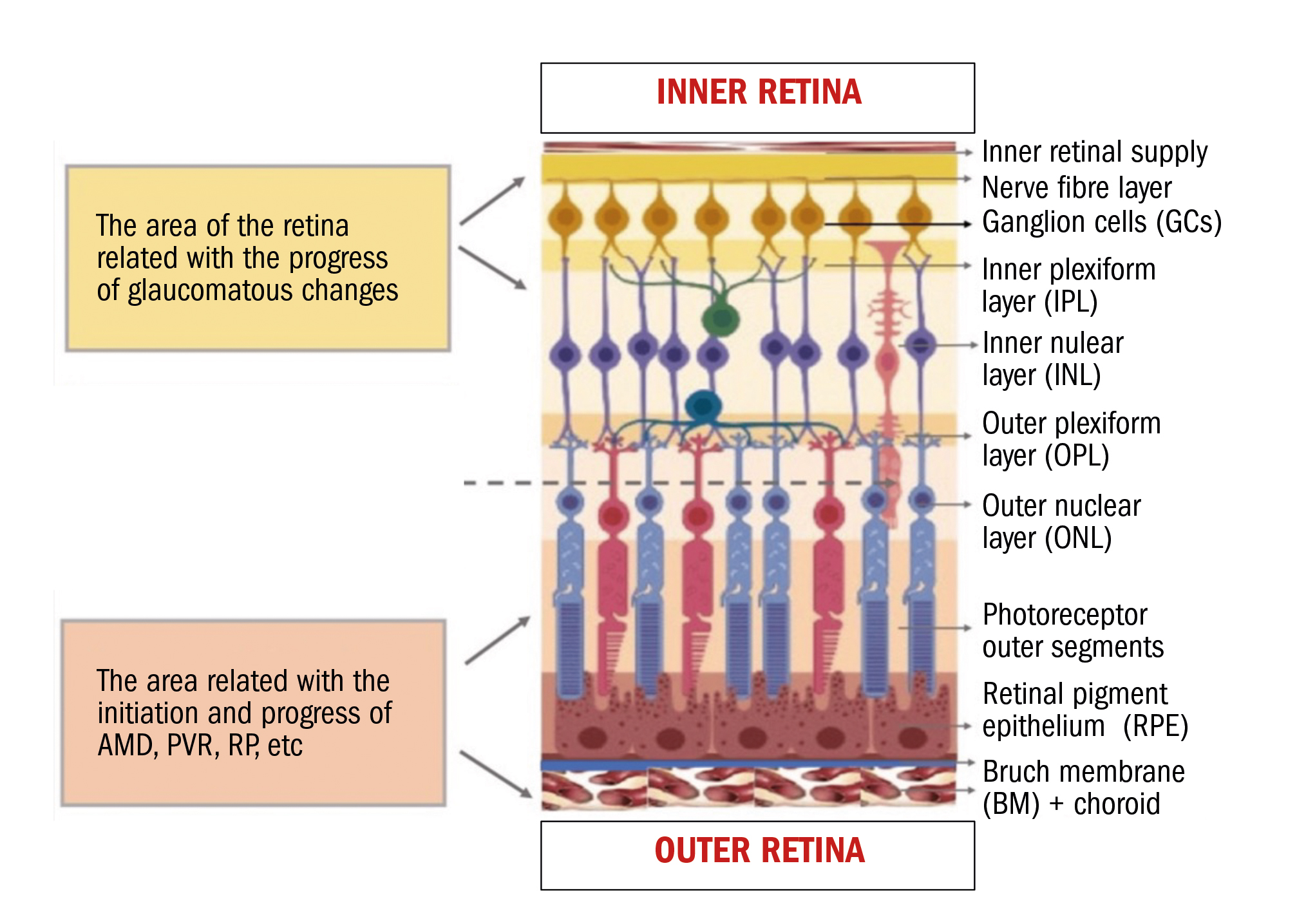
Figure 4: Areas of damage from varying pathologies within the retinal layers
The innermost five layers of the retina can also be considered as forming the ganglion cell complex (GCC) (except for the ILM), though some sources and OCT devices suggest only the RNFL, GCL and IPL compose the GCC,9 or just the RNFL and GCL.
Others, in contrast, exclude the RNFL and consider the GCL and IPL as most important to measure. Ultimately, we must consider that the retinal ganglion cell is a neuron, and, as such, it is connected from the middle retina via dendrites and synapses and sends signals to the brain via axons (the RNFL). It is the neuron that becomes ‘sick’ in glaucoma and the main body is the GCL, the dendrites are primarily the IPL layer and the axons are the RNFL.
The GCC comprises the only layers of the retina affected in glaucoma. Measuring the thickness of these layers and comparing those measurements to normative data can indicate the early signs of the disease. However, as we shall see in a later article, there are issues with the sensitivity and specificity of OCT normative databases that have led to many false positive (or unnecessary) referrals for glaucoma.
Glaucoma and optic neuropathies tend to cause thinning and damage within the inner retina.
You will also see that the outermost five layers of the retina are avascular (they should not contain blood vessels).7 The avascular retina gets its nourishment from giant Müller cells and the choroid. At the macula, because of the reduction of retinal vessels and lack of inner retina at the fovea, these areas are more dependent on the vascular support of the choroid.
This is one reason why AMD (macular degeneration) occurs, as there is only one blood supply to the macula from the choroid and a range of physiological changes, such as thickening of Bruch’s membrane, for example, can lead to the condition.10, 11
Conditions like AMD and RP (retinitis pigmentosa) tend, therefore, to cause damage within the outer retina. To understand the B-Scan a little better, it is worth understanding the more complex anatomy of the rods and cones.
As can be seen from figure 5, the outer most part of the photo receptors (outer segments) are at the bottom of the image (as in the B-Scan and anatomical diagrams). These ultimately intermingle with the projections of the RPE cells. The zone between the outer and inner segments does not show up well on OCT images and does not truly represent the real histological anatomy.
Figure 5: Anatomy of the rods and cones
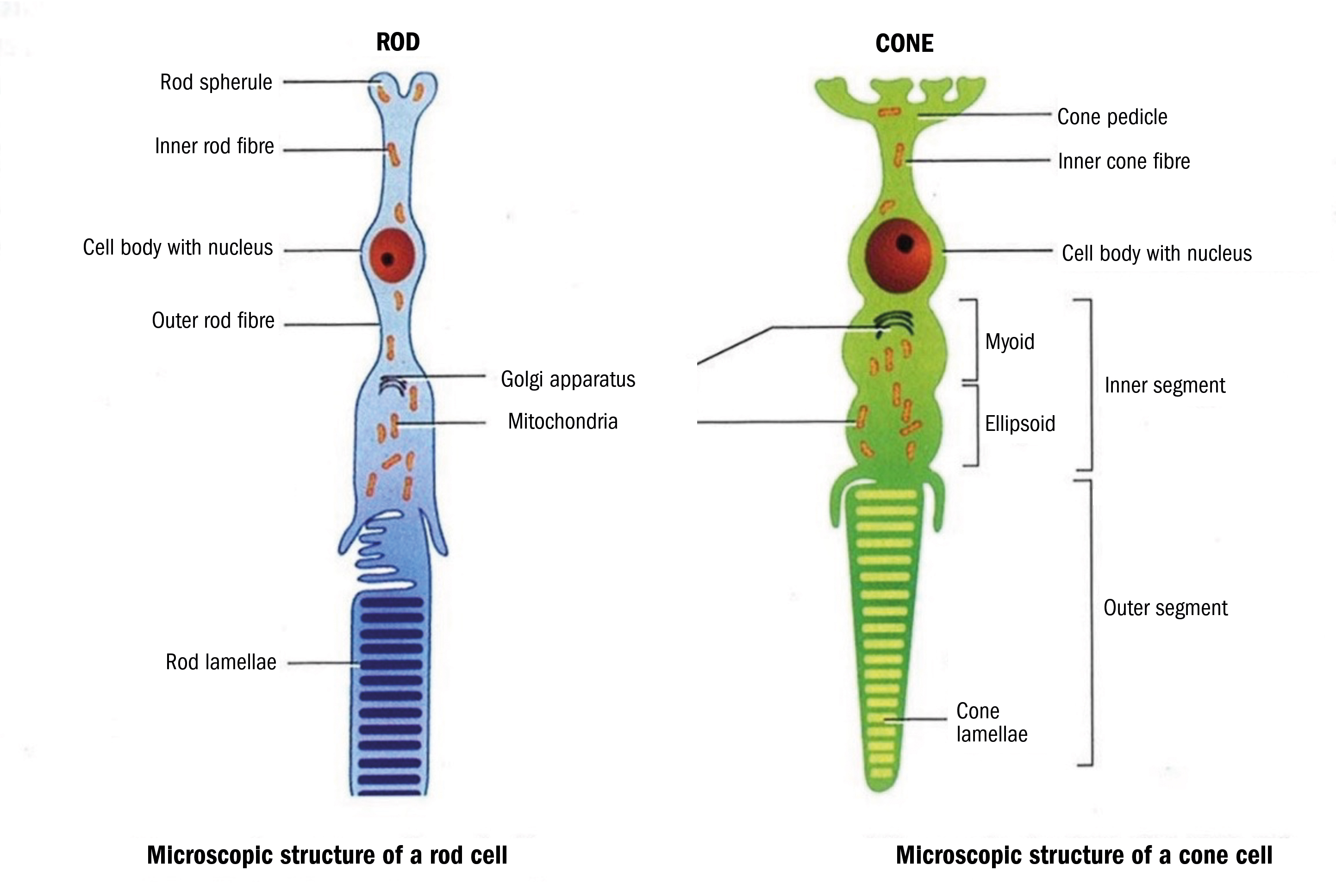
The cell body and nucleus are found in the outer nuclear layer and the synapses at the inner most end of the receptors connect to bipolar and horizontal cells in the outer plexiform layer.
It is also worth taking another look at the anatomy of the optic nerve head (ONH) or optic disc. OCT images and assessment of the ONH can lead to early detection of glaucoma but can also help identify a range of lesions and ocular conditions including papilloedema and disc drusen, for example.
In figure 6, you can see the opening in Bruch’s membrane labelled. OCT software typically uses this opening to demarcate the disc or ONH margin. When we as clinicians view the ONH directly with fundoscopy or on colour fundus imaging, we cannot, of course, see this opening. We see the inner most layers of the ONH and we use this margin as our demarcation of the outer edge of the disc.
Figure 6: Optic Nerve Head (Disc) cross section – Adobe stock licenced – labelled by author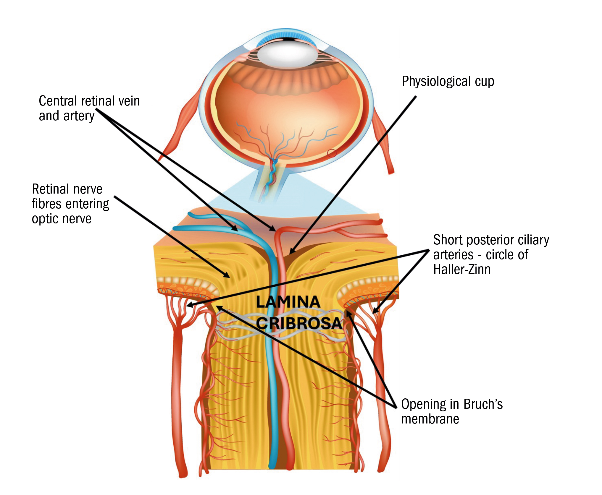
This is why OCT software always produces a larger CD ratio (cup to disc ratio) than we ourselves estimate. Both the clinician and the OCT tend to estimate the size of the cup the same, but because the OCT ONH diameter is invariably smaller from the nature of ONH anatomy, the OCT software CD ratio is higher.
The Retinal B-Scan
In figure 7, we can see a classic B-Scan of a healthy retina. The scan ‘depth’ is the distance between the top and the bottom of the image. Most OCTs found in everyday optometry practice have a scan depth of around 2.2 to 2.4mm, but some newer devices have depths of up to 12mm.
You can see that, in this classic ‘positive’ BW (black and white) B-Scan image, some layers are brighter (more hyper-reflective) and some layers are darker (more hypo-reflective). This is due to the composition of each layer, in terms of cell bodies versus nerve fibres or pigment content, for example.
Most of the labelled structures will be familiar to you and the image will look very similar to anatomy diagrams you will have encountered in your careers. One or two areas may be new to those who have not used OCT before.
RPE/Bruch’s complex (as described by Staurenghi et al12 – the IN OCT Consensus) was previously seen as a single layer considered to be the RPE. Bruch’s membrane is so thin and tightly adhered to the RPE that it is sometimes not possible to see a separation between these two distinct layers.
On more modern, higher resolution OCTs, there is often a dark (hyporeflective band) between the two layers. In pathology, Bruch’s membrane may be more apparent, such as in PED (pigment epithelial detachment) or GA (geographic atrophy).
Figure 7: Cross sectional image of a left eye OCT B-Scan. Taken from a Nidek RS-330 OCT, labelled by the author
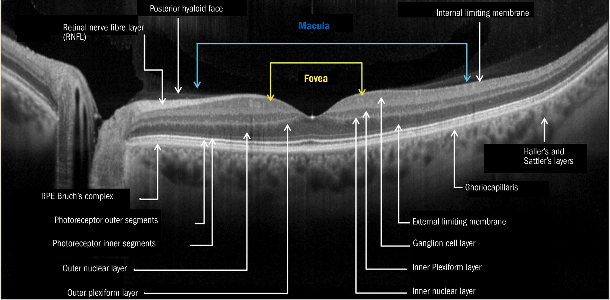
In figure 7, at the centre of the fovea (the foveola and umbo), you can see that the photoreceptor outer segments are thicker. This is due to several factors:13
- There is greater mitochondrial density in the cones here.
- Cone outer segments are elongated here due to the highest turnover of photopigment.
- The reflectance properties are altered here due to increased cone density.
You’ll also notice a bright ‘spot’ just at the base of the foveal pit. This is due to significant reflection as the infra-red laser is perpendicular to the almost flat ILM here. Seeing this bright reflection is an ‘artefact’ and is not of clinical significance in general, though it may be brighter in younger individuals and may also represent the tighter adherence of the vitreous face where ERM may be present (Tsunoda et al, 2012).
In figure 8, you can see some perhaps less familiar terminology for some areas.
Figure 8: Cross sectional image of a left eye OCT B-Scan including vitreous structures and other zones often delineated on higher resolution modern OCTs
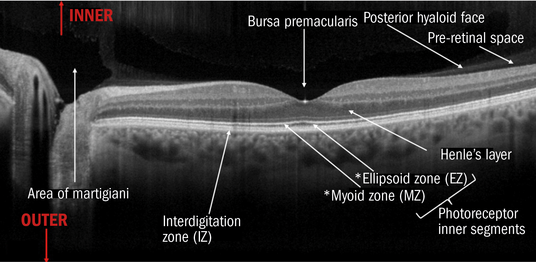
Firstly, to re-emphasise the nature of ocular anatomy terminology, it is important to remember that the OCT signal comes down from what we see as the top of the image from the front and interior of the eye outwards to the back of the eye. So, on B-Scans, the further toward the top of the image a structure lies, the further inward that structure is and vice versa.
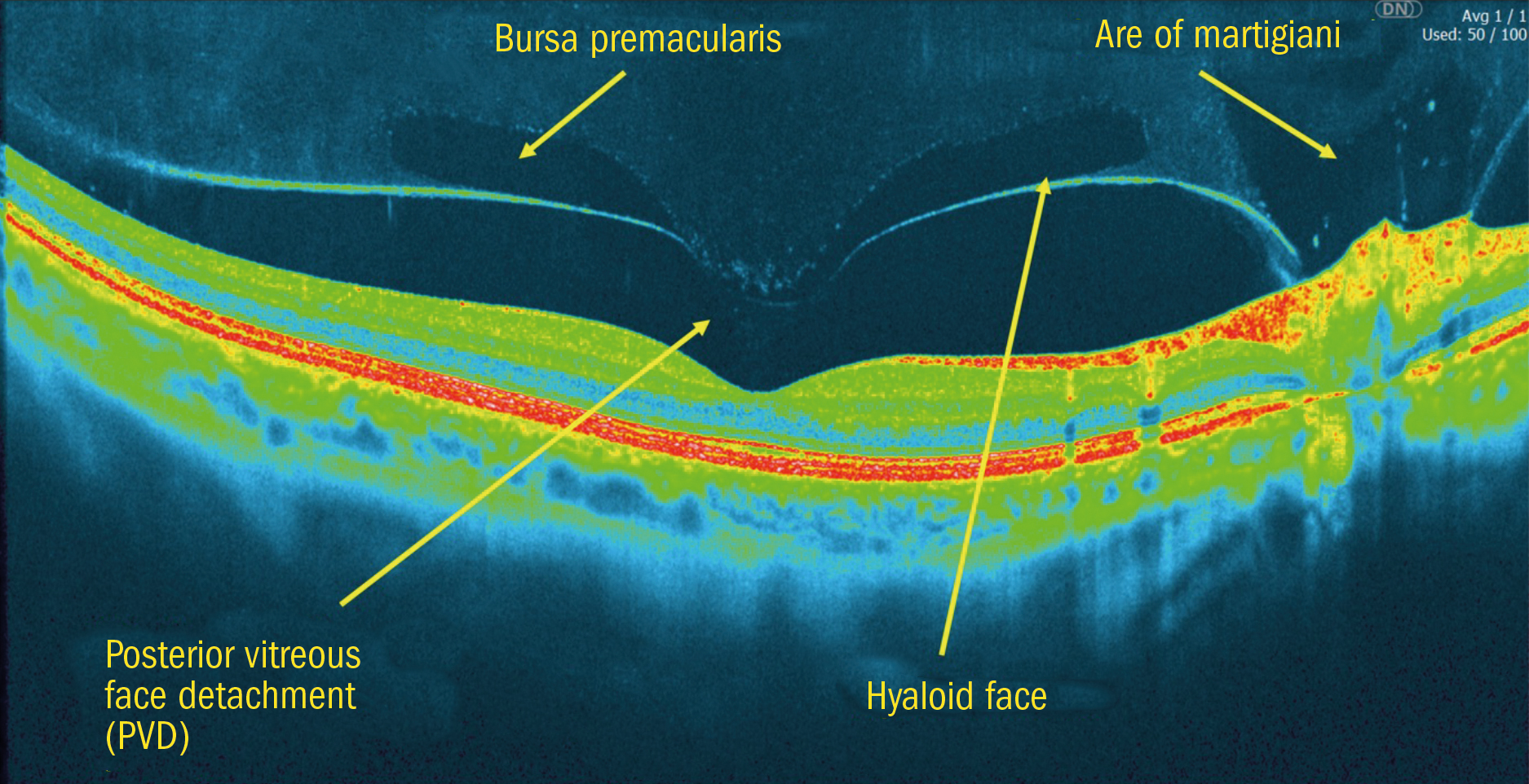
There are some vitreal structures that can sometimes appear on B-Scan images (they are often more visible on false colour scans – figure 9). The Bursa Premacularis is a physiologically normal part of the vitreous that is sometimes mistaken for a PVD (posterior vitreous face detachment). Figure 9 shows the difference in a false colour image where a PVD has taken place, and the Bursa is shown inner to the hyaloid face of the vitreous as expected.
Figure 9: False colour B-Scan showing a PVD with the Bursa inner to this
In figure 8, you will also notice three ‘zones’. According to the IN-OCT nomenclature paper: ‘The term “zone” is needed when it has better applicability to the description of tissue components. This helps to deal with regions of tissue that cannot be clearly delineated from each other with present technology.
This can occur when an OCT feature is seen to be localised to a particular anatomic region, but the specific reflective structure has not been definitively proven or because the anatomic layers are inseparable owing to interdigitation of cellular structures and tissues (eg RPE/Bruch’s complex).’
The ellipsoid zone refers to the photoreceptor outer segments and the anatomical area of the cones on histological slides. The thickness of this zone could act as a biomarker or prognostic tool in ocular diseases like vitelliform dystrophy.14
The myoid zone refers to the anatomical element of the inner segments of the photo receptors that contain a high concentration of mitochondria and Golgi apparatus.15
The interdigitation zone refers to the junction between the RPE and the outer segments of the photo receptors. On older OCTs, this was barely if ever visible, so, until the highest resolution devices are commonplace, the nomenclature refers to this as a zone as it is not a distinct layer.12
On histological diagrams, the outer nuclear and outer plexiform layers are about the same thickness, whereas on OCT, the ONL is considerably thicker than the OPL. It is suggested this is because the resolution of most OCTs is not high enough and the nature of the axonal material is lacking reflectivity to show that part of the ONL is in fact OPL. This area of axons within the OPL is sometimes referred to as Henle’s layer and should really be considered part of the OPL.12
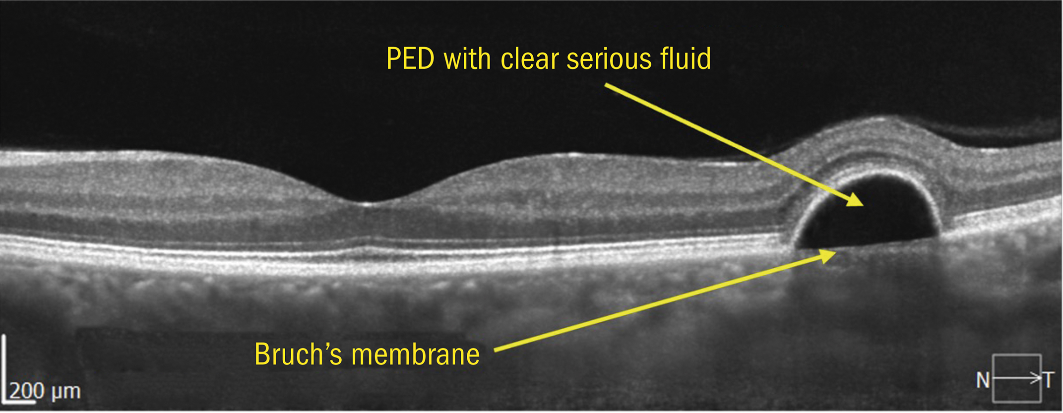
Figure 10: PED showing Bruch’s membrane separately from RPE
SD-OCT shows the choroid in reasonable detail, and it is possible to understand different layers in some detail.
As already mentioned, it generally not possible to see Bruch’s membrane in isolation in a healthy normal retina. Normally, if Bruch’s is visible separately, pathology exists. In the image below, we can see a PED (pigment epithelial detachment) where the RPE and the rest of the retina are lifted anteriorly away from Bruch’s membrane.
If we look at figure 11, we will see that the choroidal anatomical layers can also be identified to some reasonable degree of detail.
Figure 11: Sattler’s & Haller’s layers of the choroid
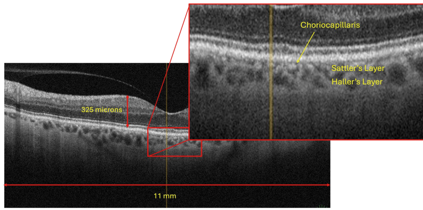
The choriocapillaris contains the microvascular connections to and from Bruch’s membrane and Sattler’s & Haller’s Layers of the choroid. The larger dark ‘voids’ within Sattler’s and Haller’s Layers are the larger arterioles and venules found in these rich vascular layers.3 Sattler’s Layer tends to have smaller and more numerous dark areas, whereas the outer Haller’s Layer has fewer such voids, but they are generally larger.
As we will see in a later article, since the advent of OCT, many new and lesser-known specific diseases of the retina and choroid have appeared. One of these has been identified by the increased central choroidal thickness at the macula area (known as pachychoroid spectrum disease).
We can also see from figure 11 that OCT B-Scans are not to scale. They are considerably vertically stretched to allow visibility of the numerous layers of the retina and to identify the smallest lesions.
It is important to remember this when viewing pathology, as sometimes, raised areas, which are quite small, may appear alarmingly substantial.
Describing OCT to Patients
There are numerous ways of describing OCT to patients, but keeping things simple and referring to the more commonly understood fundus image is a good method.
Ask the patient to ‘imagine that the colour fundus image is the icing on a cake viewed directly from above. We know that there are layers underneath, but with these two-dimensional “top-down views”, we cannot see these layers.
‘OCT allows us to take a “slice through the cake” and turn the cake on its side so we can view the layers in detail. This allows us to detect many eye conditions years before they might otherwise be identified.’
Most patients seem to understand this description easily. Many practitioners also go through the OCT results with patients, which helps them to further understand the results.
- Jason Higginbotham is an optometrist and dispensing optician with 35 years’ experience in the field. He now has his own consultancy business, FY Global Consulting, where he provides advice to multiple clients on a wide range of topics, from R&D and procurement, clinical training and education to business growth and regulations, and more besides. Jason is also the managing editor of myopiafocus.org and continues to be involved in numerous post graduate projects.
References
- Grigoryan, Eleonora N. 2022. “Cell Sources for Retinal Regeneration: Implication for Data Translation in Biomedicine of the Eye” Cells 11, no. 23: 3755.
- Yonetsu, T, Jang, I. Cardiac Optical Coherence Tomography: History, Current Status, and Perspective. JACC: Asia. 2024 Feb, 4 (2) 89–107.
- Bodenbender, J, Kowalski, M, Stingl, K, Ziemssen, F, & Kühlewein, L. (2023). Impact of A-Scan Rate on Image Quality and Acquisition Time in OCT. Current Eye Research, 48, 973 - 979.
- Thomas, B, Galor, A, Nanji, A, Sayyad, F, Wang, J, Dubovy, S, Joag, M, & Karp, C. (2014). Ultra high-resolution anterior segment optical coherence tomography in the diagnosis and management of ocular surface squamous neoplasia..The ocular surface, 12 1, 46-58 .
- Pircher, M, Hitzenberger, C, & Schmidt-Erfurth, U. (2011). Polarization sensitive optical coherence tomography in the human eye. Progress in Retinal and Eye Research, 30, 431 - 451.
- Gloesmann, M, Hermann, B, Schubert, C, Sattmann, H, Ahnelt, P, & Drexler, W. (2003). Histologic correlation of pig retina radial stratification with ultrahigh-resolution optical coherence tomography. Investigative ophthalmology & visual science, 44 4, 1696-703.
- Schmetterer, L. (2016). Retinal vasculature structure and function. Acta Ophthalmologica, 94.
- Horii, T, Murakami, T, Nishijima, K, Sakamoto, A, Ota, M, & Yoshimura, N. (2010). Optical coherence tomographic characteristics of microaneurysms in diabetic retinopathy. American journal of ophthalmology, 150 6, 840-8.
- Pazos, M, Biarnés, M, Blasco-Alberto, A, Dyrda, A, Luque-Fernández, M, Gómez, A, Mora, C, Millá, E, Muniesa, M, Antón, A, & Díaz-Alemán, V. (2020). SD-OCT peripapillary nerve fibre layer and ganglion cell complex parameters in glaucoma: principal component analysis. British Journal of Ophthalmology, 105, 496 - 501.
- Chong, N, Keonin, J, Luthert, P, Frennesson, C, Weingeist, D, Wolf, R, Mullins, R, & Hageman, G. (2005). Decreased thickness and integrity of the macular elastic layer of Bruch’s membrane correspond to the distribution of lesions associated with age-related macular degeneration. The American journal of pathology, 166 1, 241-51.
- Lim, L, Mitchell, P, Seddon, J, Holz, F, & Wong, T. (2012). Age-related macular degeneration. The Lancet, 379, 1728-1738.
- Staurenghi G, Sadda S, Chakravarthy U, Spaide RF; International Nomenclature for Optical Coherence Tomography (IN•OCT) Panel. Proposed lexicon for anatomic landmarks in normal posterior segment spectral-domain optical coherence tomography: the IN•OCT consensus. Ophthalmology. 2014 Aug;121(8):1572-8.
- Pakdel, A, Mammo, Z, Lee, S, & Forooghian, F. (2018). Normal Variation of Photoreceptor Outer Segment Volume With Age, Gender, Refractive Error, and Vitreomacular Adhesion.