Domains and learning outcomes (C111348)
• One distance learning CPD point for optometrists and dispensing opticians.
• Clinical practice
Upon completion of this CPD, ECPs will be able to describe the structure and composition of polarising filters (s5)
Upon completion of this CPD, ECPs will be able to describe scenarios in which use of polarising filters would be most useful (s5)
Building upon the initial considerations of French physicist Étienne-Louis Malus,1 the concept leading to the development of the original polarising filter, which eventually evolved into the first iteration of the polarised sunglass lens, was first introduced in the 1930s by American scientist Edwin Land (1909-1991).2
Since then, polarised sunglass lenses have been successfully used, on a global scale, to reduce reflected glare for a variety of patients, including professional sports players, amateur anglers and frequent vehicle drivers.
The aim of this article is to, first, set out the scientific background relevant to understanding what polarisation is and, second, to explore exactly how and why polarised sunglass lenses are so successful at reducing solar reflective glare.
Having a rich understanding of what visible light is made up of and how a linear polariser works is fundamental for all eye care professionals (ECPs). This knowledge will allow them to make science-based recommendations to patients who regularly complain of reflective glare affecting their ability to drive and/or their sporting performance.
Furthermore, when discussing their spectacle lens options, many patients are naturally curious to learn more about why polarised sunglass lenses would be a better option for them, over a comparatively cheaper conventional tinted sunglass lens. Therefore, a thorough comprehension of the topic of polarisation will be required to persuasively explain the key benefit that polarised sunglass lenses offer.
What is electromagnetic radiation?
In this particular context, the term ‘electromagnetic’ (EM) refers specifically to a wave that has a constantly varying electric and magnetic field, as displayed in figure 1. The electric field, E, is measured in volts per metre (V/m), and the magnetic field, M, is measured in Tesla (T).
The varying M field must propagate in a direction that is perpendicular to the varying E field. Despite being perpendicular to one another, the E and M fields must both oscillate away from their emitting source.
Finally, in this setting, the term ‘electromagnetic radiation’ (EMR) refers to a transverse EM wave that propagates in a direction that is orthogonal to both its E and M fields. The direction of travel of an EMR wave moving through space, after emission from its specific source, is demonstrated in figure 1.
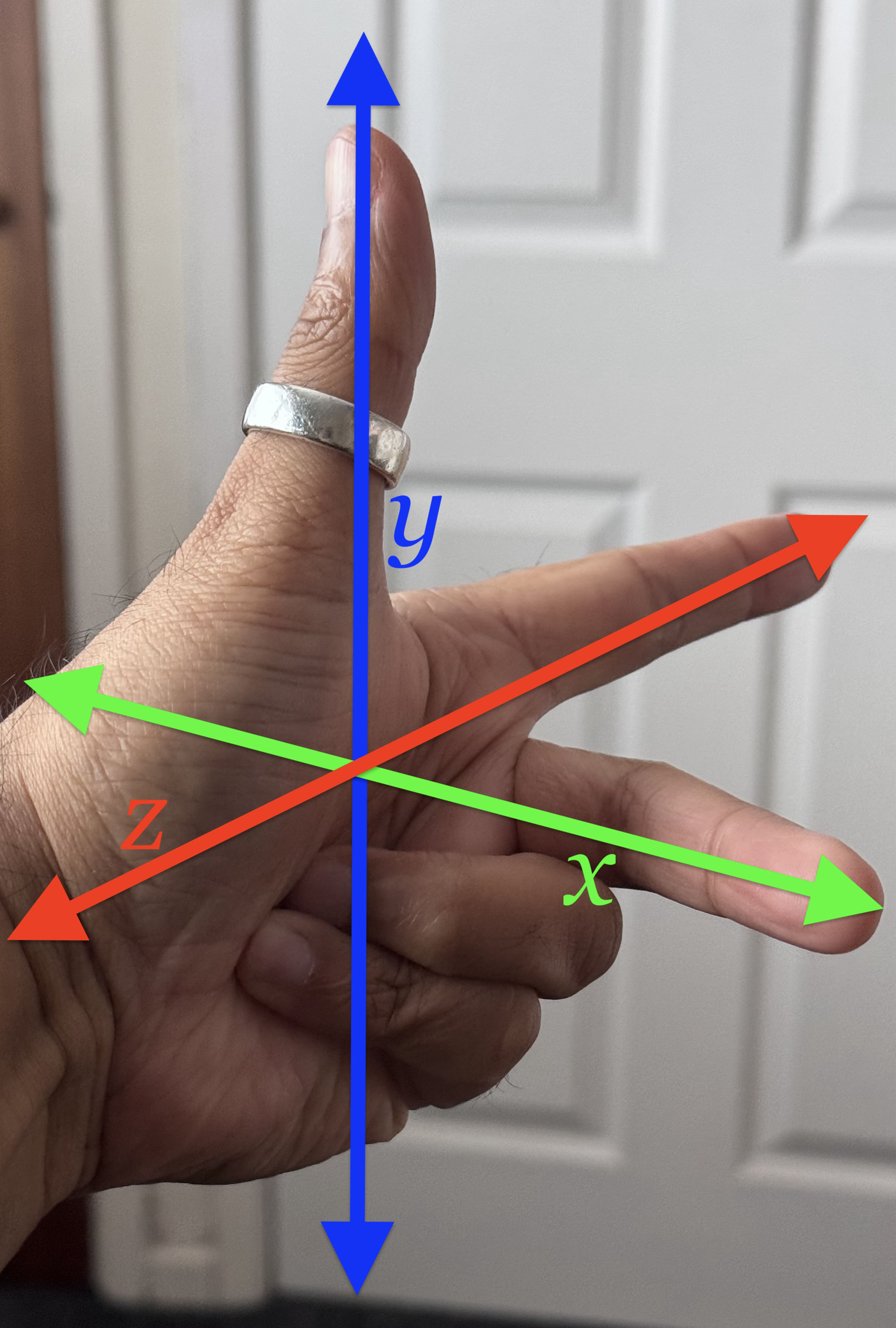
The green arrow confirms that the EMR is propagating along the direction of the X-axis. Figure 2 (below) further illustrates how all three axis directions, X, Y and Z, are perpendicular to one another.
Figure 1: A schematic of an electromagnetic (EM) wave travelling through space, which shows the relationship between the electric (E) field and magnetic (M) field oscillations. Both the E (shown in blue, travelling along the Y-axis) and M field components (shown in red, travelling along the Z-axis) are perpendicular to the wave’s direction of propagation (shown via the green arrow, travelling along the X-axis). Overall, this characteristic oscillating pattern is described as a ‘transverse’ EM wave. Visible light is an example of a transverse EM wave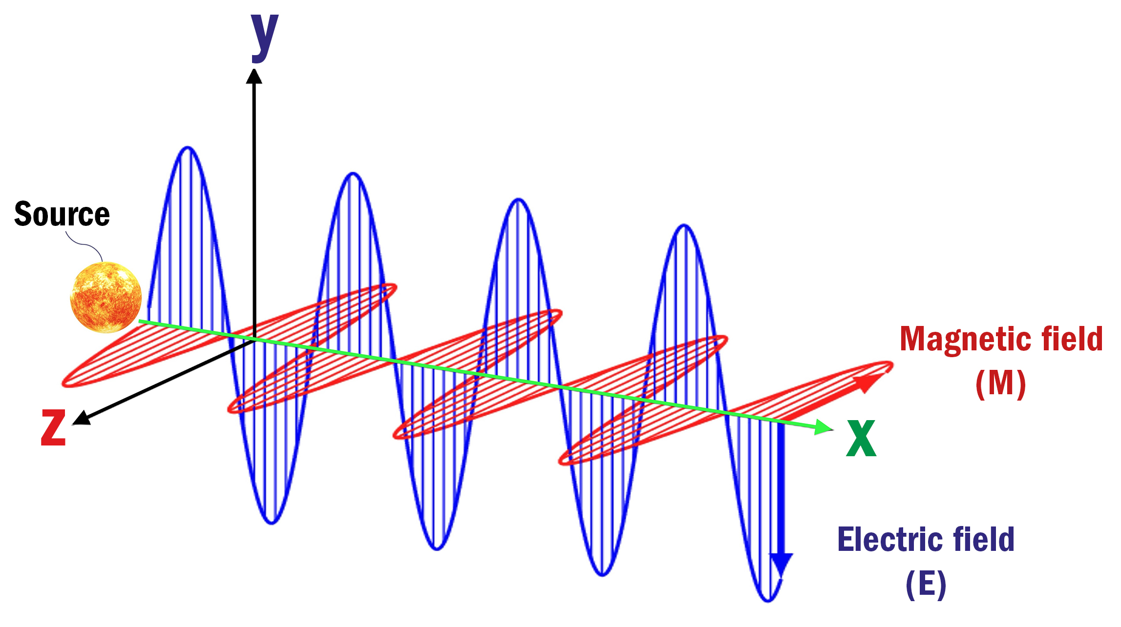
What is visible light?
Ahead of defining what polarisation is, it is critical for readers to fully grasp what visible light is and how it behaves when it interacts with physical matter.
According to Sliney,3 the wavelengths of visible light range somewhere between a lower limit of 360 and 400 nanometres (nm), up to an upper limit of somewhere between 760 and 830nm, on the EMR spectrum. The variation in values is attributable to an observer’s age, which ultimately governs the clarity of one’s crystalline lens.
British mathematician Sir Isaac Newton (1643-1727) initially theorised that visible light consisted of small particle-like bodies, called ‘corpuscles’, which had a negligible mass and were emitted by any given luminous source.4 Given Newton’s established reputation at that time, his ‘corpuscular theory’ proved to be reasonably popular for many years; however, Dutch physicist Christiaan Huygens (1629-1695) disagreed with Newton’s explanation.
In similarity to French mathematician René Descartes5 (1596-1650), Huygens proposed that light typically behaved as a wave.6 In 1804, British polymath Thomas Young (1773-1829) published the results of his famous two-slit experiment,7 which ultimately supported Huygens’ original wave propagation theory.
In his seminal 1905 publication, the Nobel prize-winning German theoretical physicist Albert Einstein remarked that,
“… when a light ray starting from a point is propagated, the energy is not continuously distributed over an ever increasing volume, but it consists of a finite number of energy quanta, localised in space, which move without being divided and which can be absorbed or emitted …”8
Fundamentally, Einstein had appreciated that visible light behaved as if it were made up of subatomic particles (initially he referred to these as ‘quanta’,8 they were, however, later renamed as photons9), and that the specific energy of each individual particle was proportionate to the frequency of its EMR.
Hence, the modern-day concept of wave-particle duality was formed, which is that quantum entities, such as the photons found within visible light, can act as both a particle and a wave, depending on the specific circumstances.
Therefore, visible light is best categorised as a form of EMR, which travels at a speed of approximately 3x10+8m/s, while propagating through a vacuum.
In summary, what an observer perceives to be a continuous wave of visible light, is actually a stream of discrete subatomic photons travelling rapidly away from the emitting source.
Which approach is the most appropriate?
‘Ray-based’ optics offers several advantages in the jurisdiction of geometrical optics, as it can be used to model and (simply) explain the major optical phenomena of refraction and reflection.
However, readers will no doubt be aware that ray-based optics simply cannot explain other more complex optical phenomena, such as diffraction, constructive interference, total destructive interference and polarisation.
As the focus of this article is on polarisation, a ‘wave-based’ approach shall be required to explain, represent and model the main optical principles underpinning polarisation.
What is polarisation?
When considering light as an EM wave in the field of physics, it is well-established that the magnitude of the E field is the most important factor when considering meaningful interactions between this form of EMR and other physical matter (e.g., a smooth reflective surface).
By contrast, the M field is of little significance. Therefore, for the remainder of this article the M field component shall be ignored accordingly.
Polarisation must be considered as a ‘physical’ property of visible light waves, just like either their amplitude or frequency. Polarisation describes the specific orientation of the direction of the EM wave’s E field oscillation as it propagates through space.
In simple terms, there are three broad categories of polarisation: unpolarised light, plane polarised light and partially polarised light. Visible light waves emitted by a luminous source, such as our Sun, are characteristically described as unpolarised.
This is because the emitted EM waves all propagate in the same direction, yet their E field oscillations are typically angled in random orientations about the axis of propagation, as depicted in figure 3A.
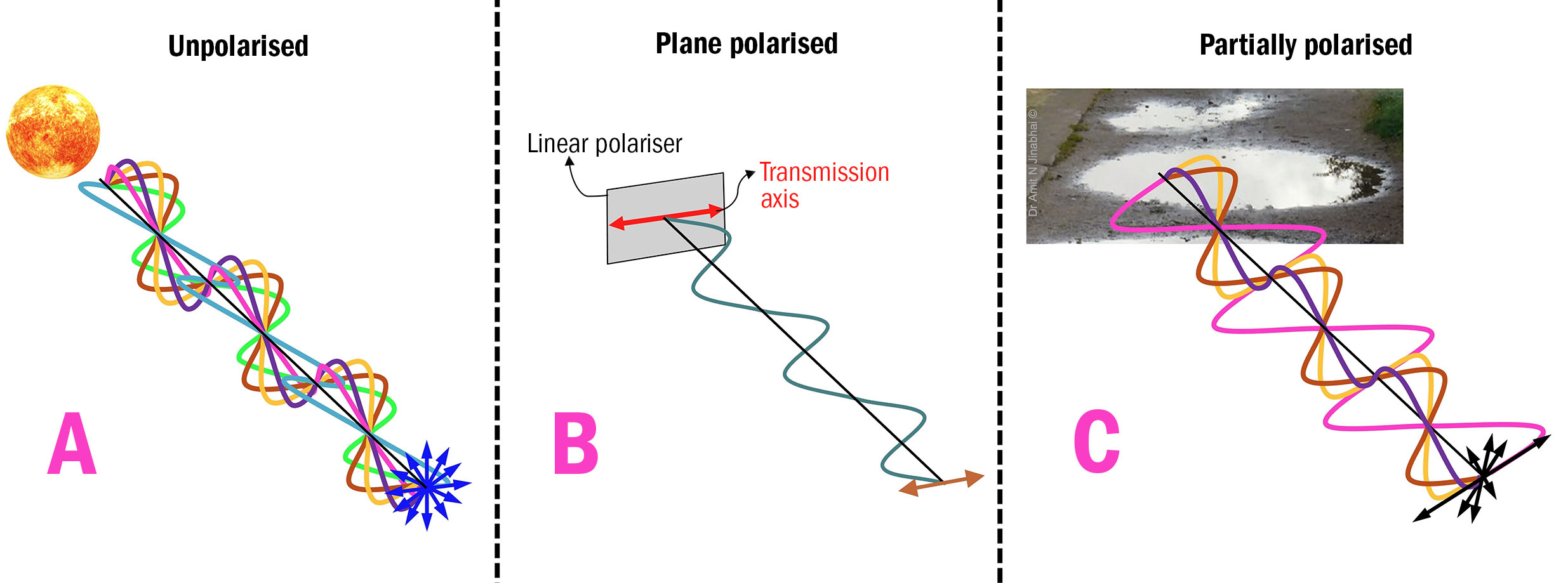
By stark contrast, plane polarised light comprises EM waves where the precise orientation of the E field’s oscillation is the same for all of the propagating waves, as shown in figure 3B. Plane polarised light is typically created by shining unpolarised light through a linear polariser.
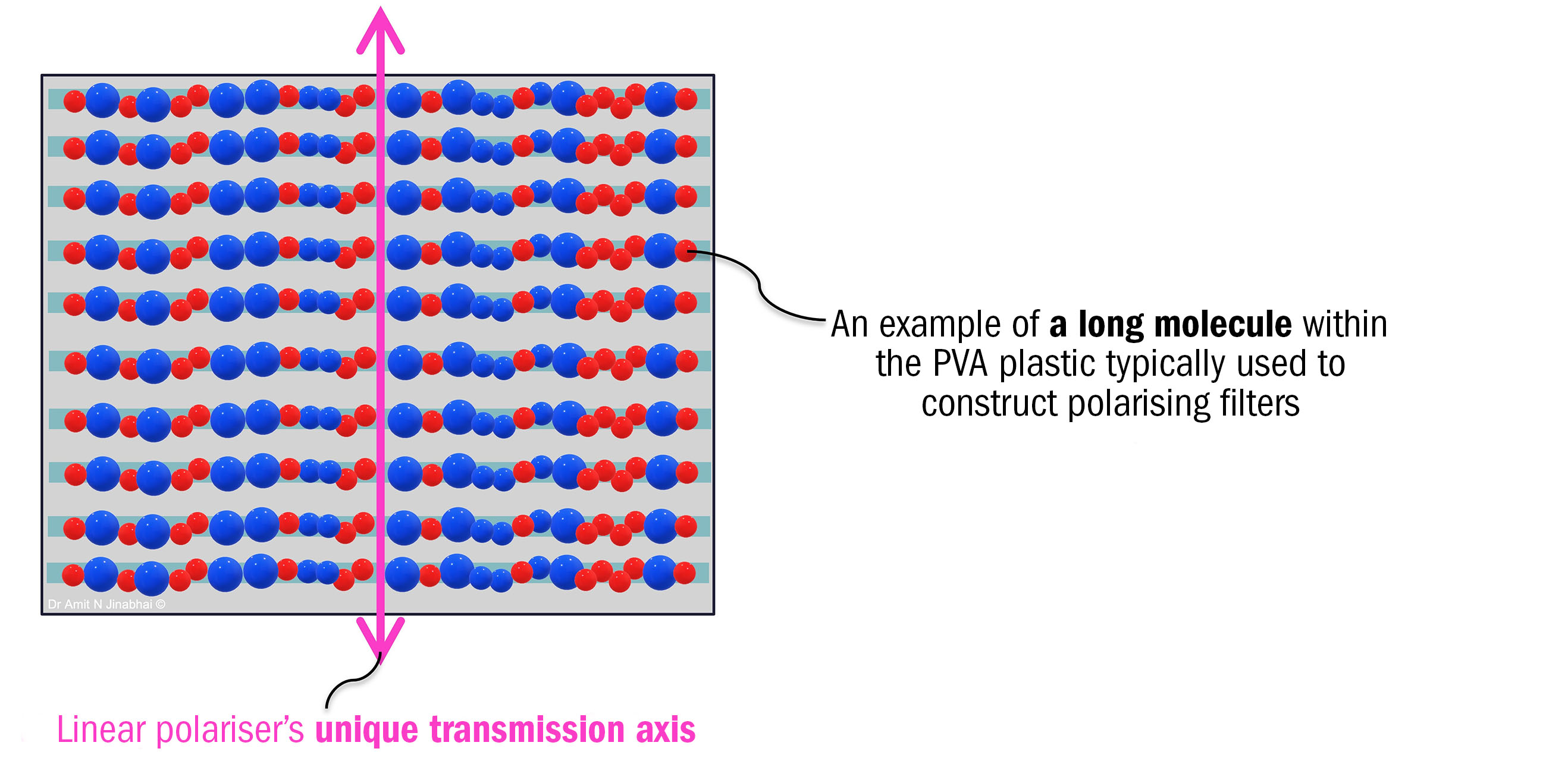
Linear polarisers (commonly referred to as ‘polarising filters’) are typically constructed from long molecules of polyvinyl alcohol (PVA) plastic that are stretched out and arranged into numerous parallel rows. This material is then impregnated with iodine. Linear polarisers have a unique transmission axis which is always positioned perpendicular to the physical orientation of the long molecular rows – see figure 4.
Figure 4: A simple schematic of the basic molecular structure of a linear polariser (polarising filter). The long polyvinyl alcohol (PVA) molecules of this particular filter are arranged into ‘rows’ that are orientated horizontally. In contrast, the polariser’s transmission axis is located vertically
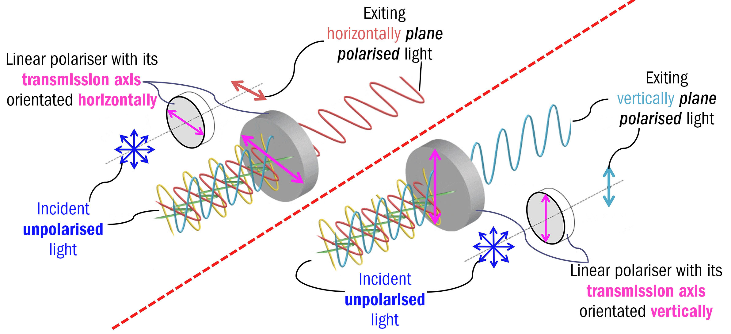
The resulting EM wave that exits from a linear polariser will be polarised along a linear plane that is exactly parallel to the polariser’s transmission axis. As illustrated in figure 5, the unique orientation of the plane polarised waves exiting from a linear polariser can be altered by simply ‘rotating’ the polariser’s orientation and hence its transmission axis.
In this figure, the transmission axis has been rotated from an initial ‘horizontal’ orientation (shown on the left-hand side of the red dashed line) to a ‘vertical’ orientation (shown on the right-hand side).
Figure 5: A schematic allowing a direct comparison between the orientation of the plane polarised light waves exiting from two differently orientated linear polarisers. This figure contains two traditional arrow-based diagrams, and two wave-based diagrams. Both methods are presented to aid the readership’s interpretation. Each linear polariser has unpolarised light incident upon it, which is depicted via the four dark-blue double arrows, and via the four individually coloured waves presented directly in front of the linear polarisers.
Below left: The transmission axes of the linear polarisers are orientated horizontally; hence, the exiting light is plane polarised horizontally (as depicted via the dark-orange-coloured double arrow and wave), ie exactly parallel to the transmission axes.
Below right: The transmission axes of these linear polarisers are orientated vertically; hence, the exiting light is plane polarised vertically (as depicted via the cyan-coloured double arrow and wave), ie exactly parallel to the transmission axes
Finally, as illustrated in figure 3C, light that reflects (via specular reflection) off the smooth surface of a transparent refractive medium (such as water in a puddle), back into air, is typically partially polarised. In this case, the reflected EM waves are all propagating in the same direction.
But, while their E field oscillations are typically angled in random orientations about the axis of propagation, the amplitude of one given orientation’s oscillation will be noticeably larger and more ‘dominant’ than that of the others – as depicted by the magenta-coloured curve in figure 3C.
In addition to the cases of transmission through a linear polariser and specular reflection (as described above), polarisation can also be achieved through refraction, via birefringent materials,10 and by scattering.11 The latter two methods fall far beyond the scope of this article.
Simplifying unpolarised light
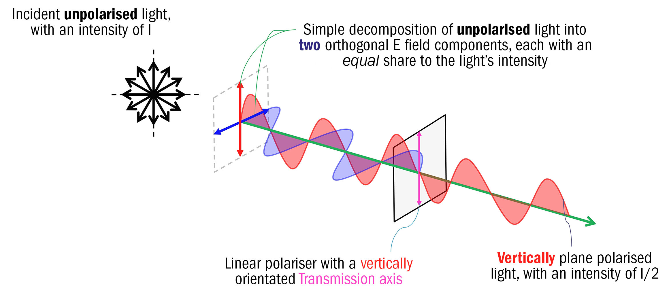
To properly interpret the polarisation state of a wave, consideration must first be given as to how unpolarised light should be characterised. An unpolarised light wave that is incident upon a linear polariser can very simply be decomposed (by way of vectors) into two orthogonal E field components that have equal amplitudes and are propagating in the same direction of travel.
One component will oscillate in a plane that is perpendicular to the polariser’s transmission axis, while the other will oscillate in a plane that is parallel to this transmission axis. This simple approach works because there is no dominant plane of polarisation within unpolarised light.
Therefore, it can be reasonably assumed that 50% of this incident light’s intensity will be carried by each of these two orthogonal components via an ‘even’ split. Using this simplistic approach, figure 6 clearly illustrates that the light transmitted by a linear polariser will have only 50% of the intensity of the incident unpolarised light.
Figure 6: A schematic depicting the oscillating electric (E) field exiting from a linear polariser whose transmission axis is orientated vertically (denoted by the magenta-coloured double arrow). As the light incident upon this polariser is unpolarised (as denoted by the six black double arrows), it can be simply decomposed into two orthogonal E field components. One component will be oscillating perpendicular to the polariser’s transmission axis (as denoted by the blue double arrow), while the other will be oscillating parallel to the transmission axis (as denoted by the red double arrow). The two E field components will have the same amplitude, will share the overall intensity in a 50:50 split, and will propagate in the same direction of travel (denoted by the green arrow). The light exiting from this linear polariser is plane polarised vertically
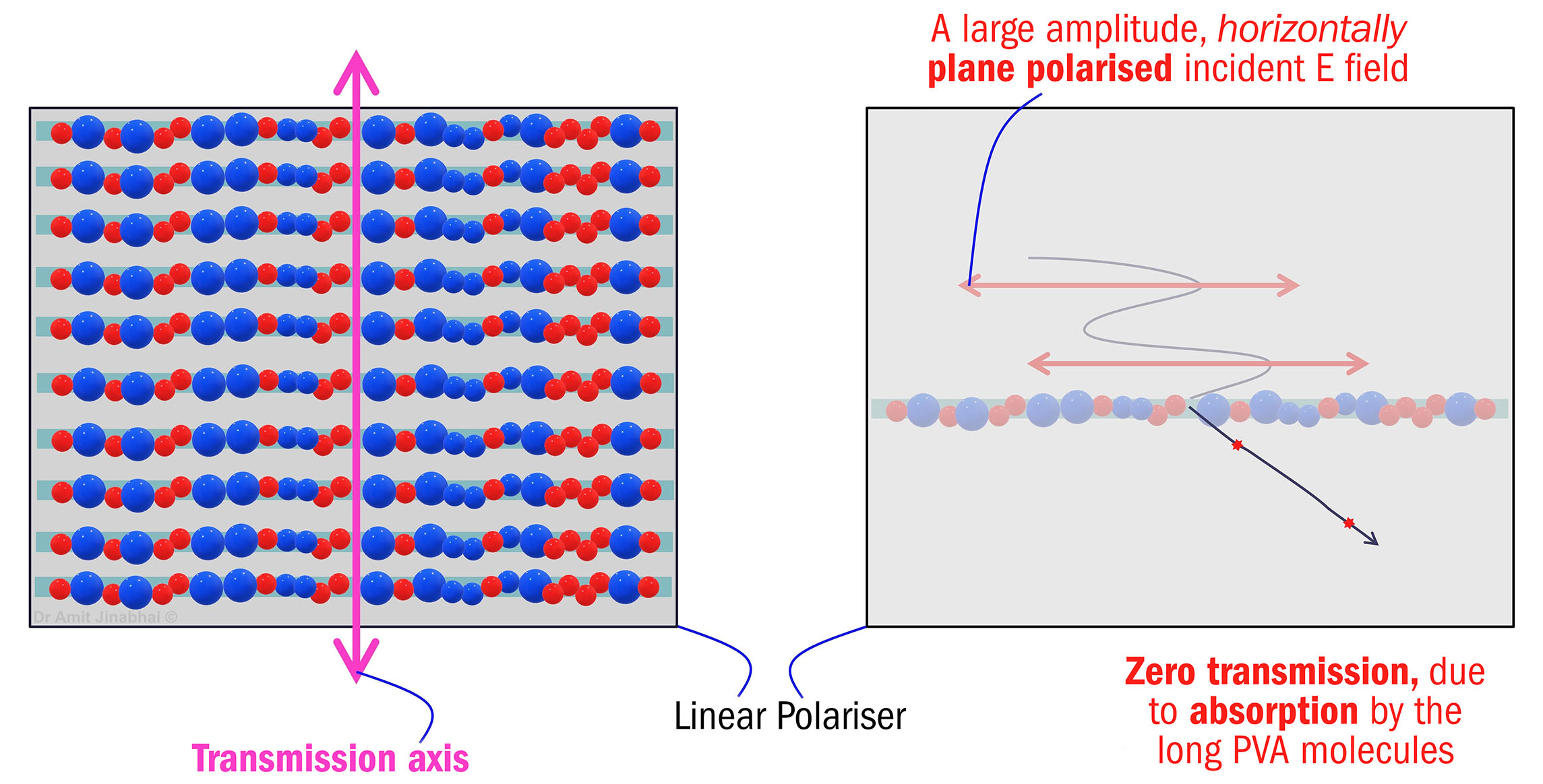
Decomposing an unpolarised light wave in this manner lends further support to understanding exactly how an E field oscillation of a particular orientation can be ‘absorbed’ or ‘transmitted’ through a linear polariser. The upper half of figure 7 demonstrates how the long rows of molecules embedded within a linear polariser are capable of easily absorbing an oscillating E field, which vibrates in a plane that is parallel to these molecules, yet perpendicular to the polariser’s transmission axis.
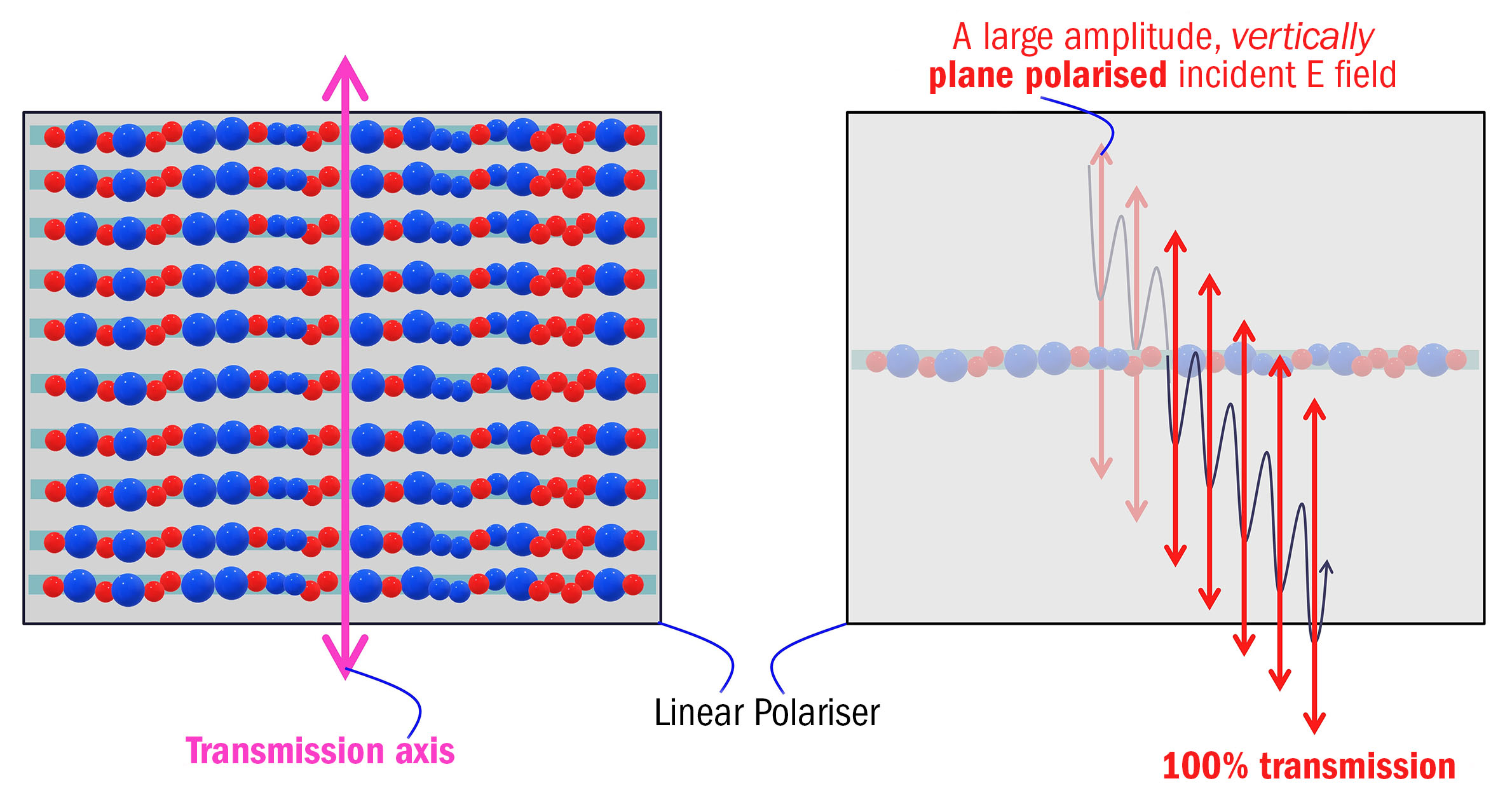
In stark contrast, the lower half of figure 7 demonstrates how an oscillating E field, which vibrates in a plane that is parallel to the linear polariser’s transmission axis (yet perpendicular to the long molecules), can easily pass through the polariser and remains unimpeded.
Figure 7: A schematic explaining how a linear polariser (polarising filter) works. In each image, the polariser’s transmission axis is located vertically.
In the two right-hand images, only one molecular chain has been shown for ease of interpretation.
Upper images: As the long polyvinyl alcohol molecules are orientated horizontally within the linear polariser, they readily ‘absorb’ the large amplitude, horizontally oscillating electric (E) field that is incident upon the polariser. Consequently, zero transmission occurs.
Lower images: The large amplitude, vertically oscillating E field incident upon the linear polariser is vibrating in a plane that is exactly parallel to the polariser’s transmission axis, which means that it very easily passes through the polariser unimpeded; therefore, 100% transmission occurs
Reflective glare off wet road surfaces
Wet road surfaces can cause drivers significant visual problems because the water-to-air surface boundary is capable of inducing significant solar reflective glare, particularly in winter, when the Sun is typically lower in the sky – see figure 8.
To help significantly reduce this specific type of induced reflective glare, ECPs are able to use their knowledge of physical optics to recommend and dispense polarised sunglass lenses, which are invaluable to those who spend a lot of their time driving.
Having set out the relevant scientific background, the focus of this article will now shift to exploring exactly how and why polarised sunglass lenses are so effective at reducing solar reflective glare off wet road surfaces.
Figure 8: A photograph showing significant glare due to sunlight reflecting off the surface water present on a UK road after a period of heavy rainfall on a sunny winter’s day. This reflected light will be partially polarised in the plane parallel to the water’s surface

Polarisation induced by reflection
In order to fully appreciate how a polarised sunglass lens works, it is important to consider the ‘plane’ in which any reflected light becomes partially polarised. Figure 9 illustrates how, whenever unpolarised sunlight reflects off the surface of water back into air, it becomes partially polarised in a plane that is parallel to the water’s surface.
By way of contrast and as an aside, unpolarised sunlight transmitted/refracted at this air-to-water boundary becomes partially polarised in a plane that is perpendicular to the water’s surface; however, this aspect (ie refraction) is not the focus of this article.
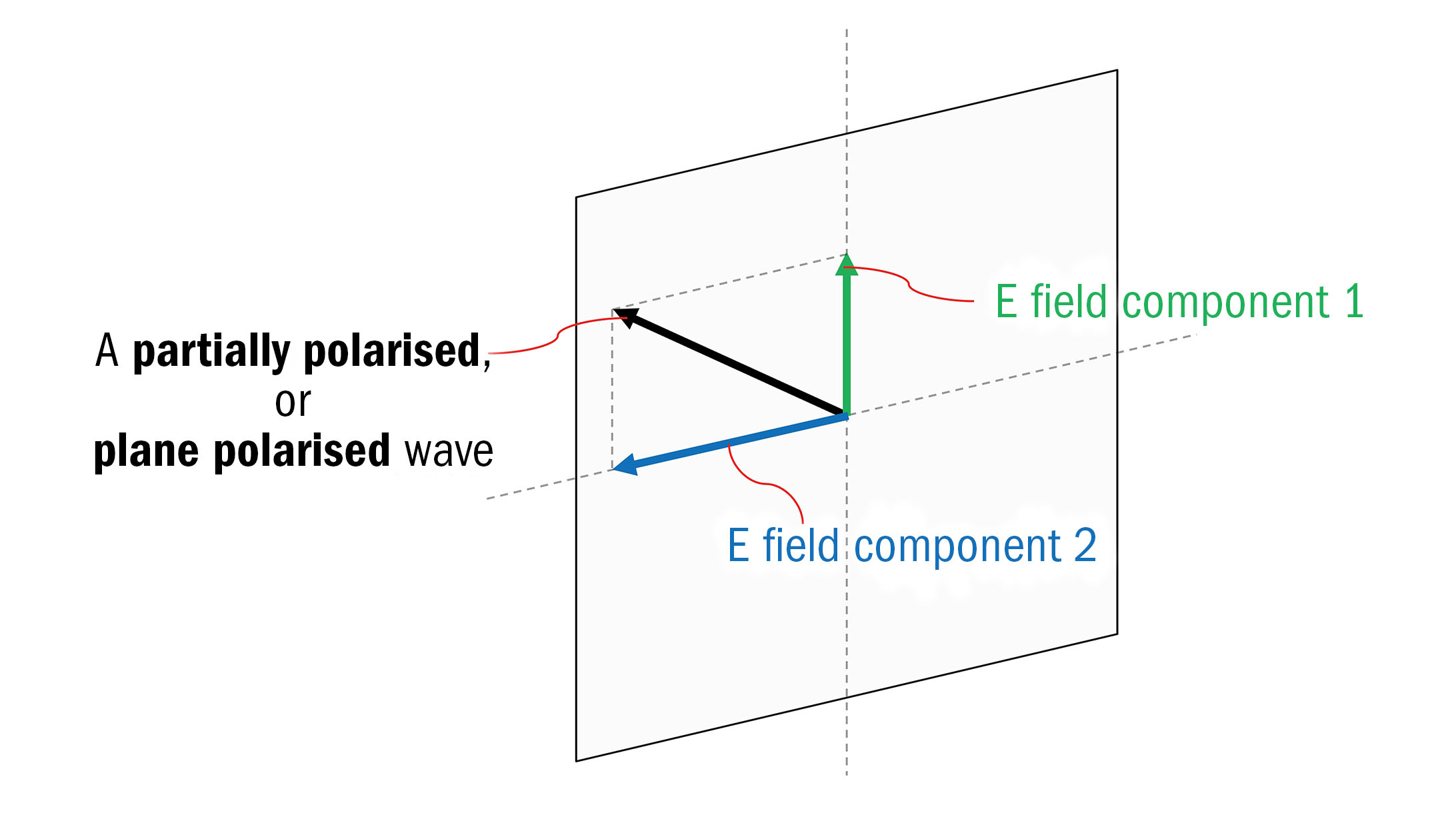
Figure 10: A diagram illustrating how a partially polarised or plane polarised light wave can be decomposed (by way of vectors) into two orthogonal electric (E) field components. In this case, the two E field components are unequal in their amplitudes. Nevertheless, both E field components will propagate in the same direction of travel
While this basic concept of polarisation by reflection is relatively simple to understand, an unavoidable degree of complexity is introduced courtesy of the formulae required to calculate the reflectance (R) of the partially polarised light at the water-to-air surface boundary. These particular formulae are attributed to Augustin-Jean Fresnel (1788-1827).12
Reflectance is the term used to quantify the fraction of the light intensity (I) that is reflected at the surface boundary. Essentially, reflectance represents the ratio of the reflected intensity and the incident intensity. It is important to recognise that the intensity of the reflected light will differ depending on its degree of polarisation.
Rather than simply considering reflection in relation to the surface boundary in question, Fresnel’s equations complicate matters by specifically computing the reflectance of light polarised perpendicular to (R⊥) and parallel to (R||) the plane of incidence (POI).
In this context, the POI is the plane that contains the propagating incident radiation, the normal line formed with respect to the reflective surface, and the propagating reflected radiation.
Fresnel’s original reflectance equations have been widely reproduced in many well-established optometry textbooks; for example, in Tunnacliffe and Hirst’s Optics.13 However, for some, these equations may be difficult to use. To update their interpretation and application, this article presents simplified versions which include the following expressions:
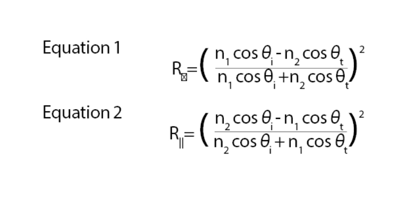
In both equations, n1 represents the refractive index of the first medium that the incident wave travels through (ie air: 1.00), whereas n2 represents the refractive index of the second medium (ie water: 1.33). Additionally, θi represents the magnitude of the incident angle, whereas θt represents the magnitude of the transmitted/refracted angle.
Helpfully, Fresnel’s equations make use of a simple, vector-based mathematical model, which considers that any partially polarised or plane polarised light wave can be treated as if it were the wave created via superposition of two orthogonal E field components – see figure 10.
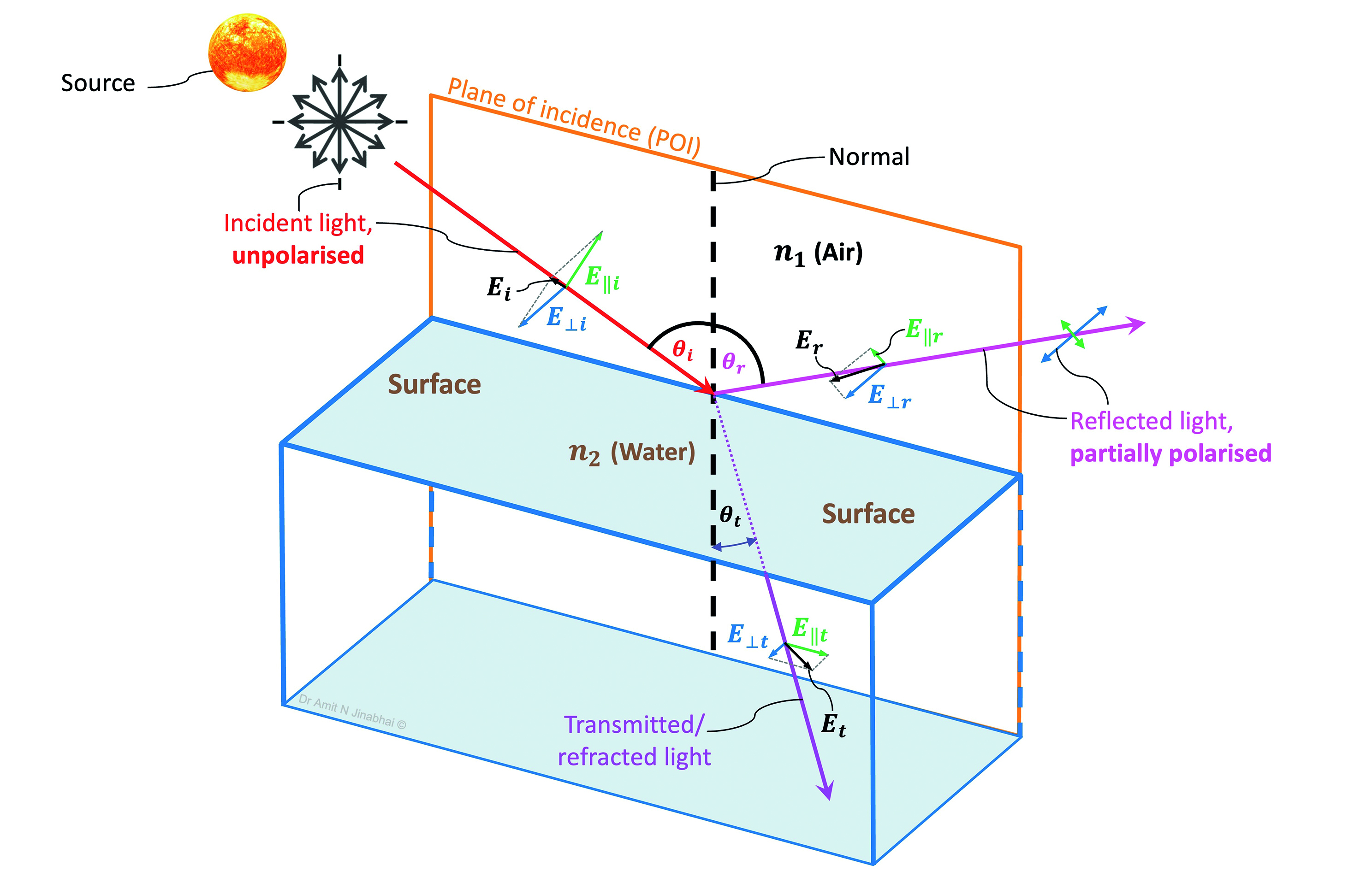
Figure 11: A schematic illustrating what happens to unpolarised sunlight (denoted by the six black double arrows) as it arrives at a smooth surface between air (n1: 1.00) and water (n2:1.33).
As described in the article and illustrated in figures 6 and 10, the incident (Ei), reflected (Er) and transmitted/refracted light (Et) have each been decomposed into two orthogonal electric (E) field components: one that is parallel (||) to the plane of incidence (POI), and one that is perpendicular (⊥) to the POI. The POI is shown in orange and is defined as the plane which contains the propagating incident radiation, the normal line formed with respect to the surface (denoted by the dashed black line), and the propagating reflected radiation.
When unpolarised incident sunlight reflects off the surface of water, at a water-to-air boundary, its E field component becomes partially polarised in a plane that is perpendicular to the POI, E⊥r. This particular orientation of polarisation is shown via the larger, blue-coloured arrows. The comparatively smaller, green-coloured arrows represents the E field component reflected parallel to the POI, E||r .
In contrast, the unpolarised incident sunlight transmitted/refracted at this interface becomes partially polarised in a plane that is parallel to the POI, E||t. This particular orientation of polarisation is shown via the large, green-coloured arrow. The comparatively smaller, blue-coloured arrow represents the E field component transmitted/refracted perpendicular to the POI E⊥t.
E⊥i : the unpolarised incident light’s E field component perpendicular to the POI; E||i : the unpolarised incident light’s E field component parallel to the POI; θi: angle of incidence (degrees); θr: angle of reflection (degrees), and θt: angle of transmission/refraction (degrees)
Both E field components will propagate in the same direction of travel. Of these two E field components, one will always oscillate perpendicular (⊥) to the POI while the other will always oscillate parallel (||) to the POI.
Figure 11 carefully illustrates how the incident unpolarised light, the water-to-air surface boundary, the location of the POI, the reflected light, and the transmitted/refracted light all fit neatly together. In this diagram, readers should also observe that the POI is essentially perpendicular to the water’s surface.
As the incident light (denoted by the red arrow) is unpolarised, the E field component perpendicular to the POI (E⊥i), will have the exact same magnitude as the E field component parallel to the POI (E||i), via a 50:50 split. Reflection then occurs at the water-to-air boundary, as denoted by the magenta arrow. This induces partial polarisation, such that the E field component perpendicular to the POI (E⊥r), as denoted by the blue arrow, will show a much larger magnitude than the E field component parallel to the POI (E||r), as denoted by the green arrow.
Therefore, it can be concluded that figure 11 illustrates how the reflected light becomes partially polarised, and that the most ‘dominant’ E field oscillation’s orientation is perpendicular to the POI (E⊥r), which, in turn, is parallel to the water’s surface.
Having established this particular orientation, Fresnel’s equations shall now be used to calculate the values for the reflectance perpendicular to the POI (R⊥) and parallel to the POI (R||).
Assuming that the refractive index of the water is 1.33, and that the angle of incidence of the unpolarised light was 50 degrees, the angle of transmission, θt, (due to refraction) can be easily deduced using Snell’s time-honoured law of refraction:14
n1× Sin(θi) = n2× Sin(θt) … rearranging this for the angle θt gives, to two decimal places:
θt=ArcSin ((1.00) × (Sin(50°))) = 35.17°
1.33
Inserting these data into Equations 1 and 2 gives: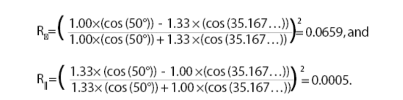
Expressing each of these raw reflectance values as a percentage, to two decimal places, confirms that the light polarised perpendicular to the POI (R⊥) has a reflectance of 6.60%, whereas the light polarised parallel to the POI (R||) has a significantly lower reflectance of only 0.05%. These key calculations confirm that the ‘dominant’ plane of oscillation, as identified in figure 11, has the higher intensity and therefore induces the greater degree of reflective glare.
Brewster’s angle
Figure 12 presents a graph of the raw reflectance values (R⊥ and R||) plotted as a function of the angle of incidence (θi). When observing this graphical relationship, readers should note that there is a specific angle of incidence where the reflectance of light polarised parallel to the POI (R||) falls to zero. This special angle of incidence is better known as Brewster’s angle, θB, named after its founder, Scottish physicist Sir David Brewster (1781-1868).15 Most importantly, at Brewster’s angle, the light reflected perpendicular to the POI (R⊥) will be truly plane polarised.
The value of Brewster’s angle for this water-to-air boundary (assumes water’s refractive index is 1.33) can be calculated using Equation 3, which gives:
Polarised sunglass lenses
All of the information presented above helps to justify why polarising sunglass lenses are extremely useful in reducing reflective glare off wet road surfaces and other bodies of water.
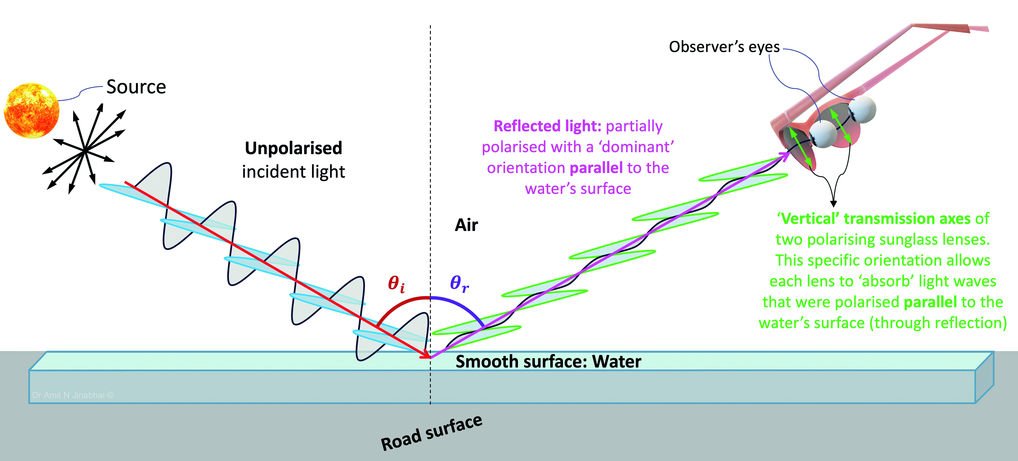
To be maximally effective, spectacle lens manufacturers must always set the transmission axes of their polarised sunglass lenses to the ‘vertical’ position, as illustrated by the magenta-coloured double arrows in figure 13. Orientating the transmission axes in this highly specific manner allows light that has become partially polarised, due to reflection off a horizontal water-to-air boundary, to be absorbed by the polarised sunglass lens.
Hence, this light does not physically reach the wearer’s retina, as illustrated in figure 14. This optical phenomenon provides an everyday practical example of how an ECP’s rich knowledge of physical optics can be utilised to significantly reduce reflective glare for their patients.
Figure 12: A plot of reflectance as a function of the angle of incidence. The blue curve represents the raw reflectance values plotted for light polarised perpendicular to the plane of incidence (POI), R⊥. The red curve represents the raw reflectance values plotted for light polarised parallel to the POI, R||. The refractive index of water was assumed to be 1.33, thereby providing a Brewster’s angle value of 53.06 degrees
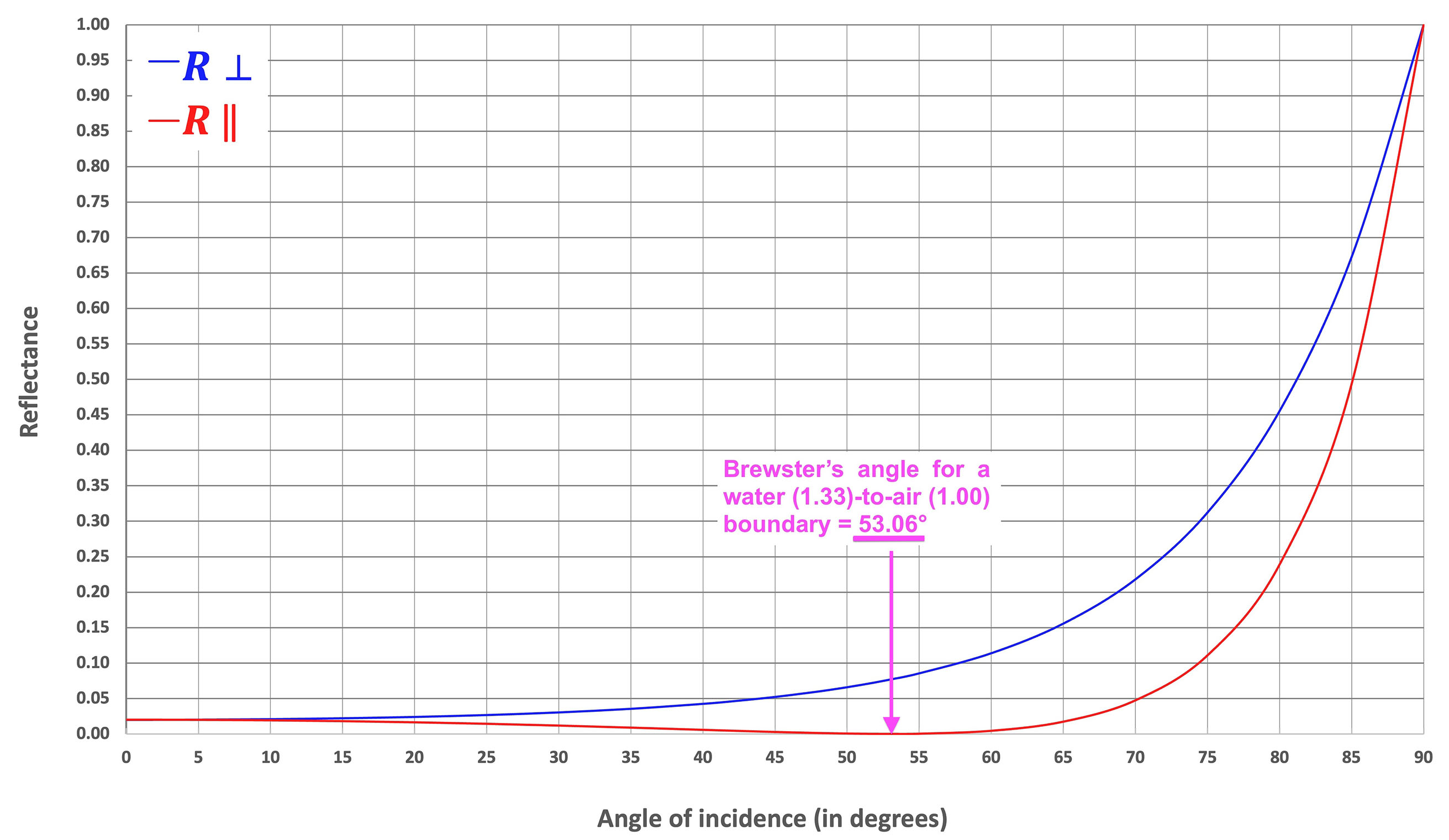
Moreover, figure 12 confirms that polarised sunglass lenses can be successfully used to reduce reflective glare from the surface of water for angles of incidence between 35 and 72 degrees. This fact emphasises that polarised sunglass lenses are an ideal solution for drivers, cyclists, anglers and sailors who may frequently complain about problematic reflective glare, off the surface of water, to their ECP.
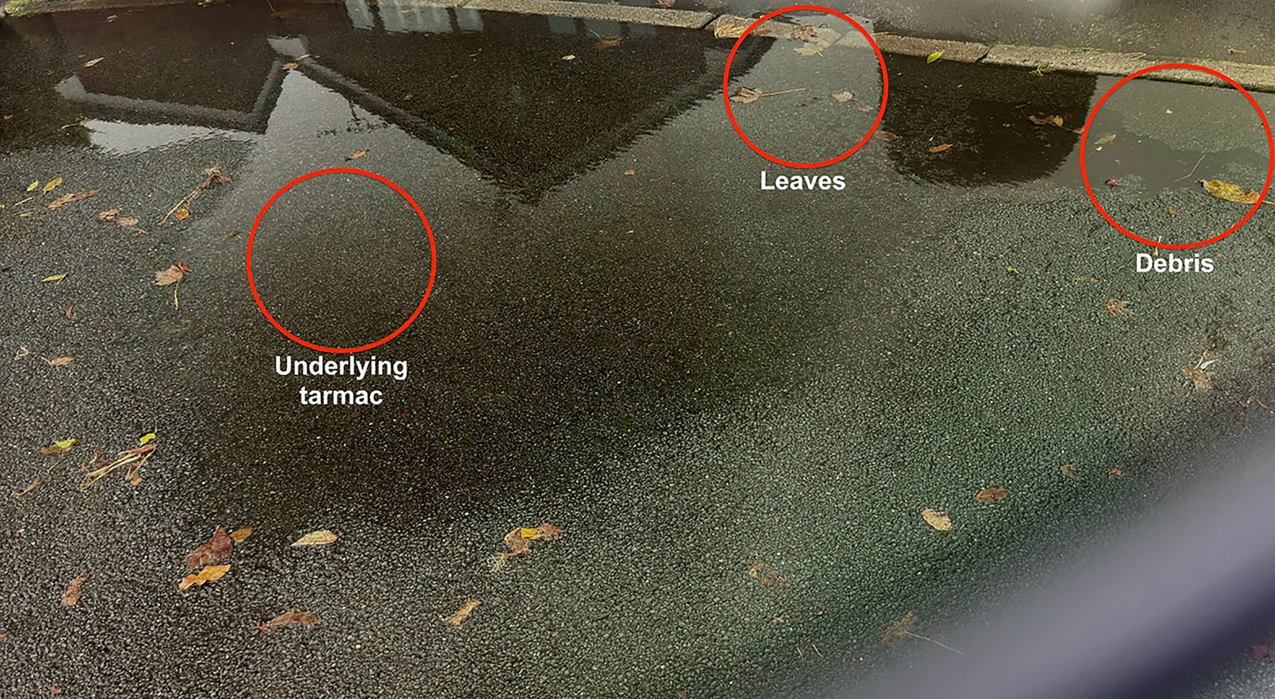
To further illustrate the effectiveness of polarised sunglass lenses, figure 15 provides a direct comparison of the reflective glare observed between photographic images of a large puddle of water shot without and with a polarised sunglass lens in situ.
Figure 13: A pair of polarised sunglasses. The transmission axis for each polarised sunglass lens must be set to the ‘vertical’ position, as depicted by the magenta-coloured double arrows
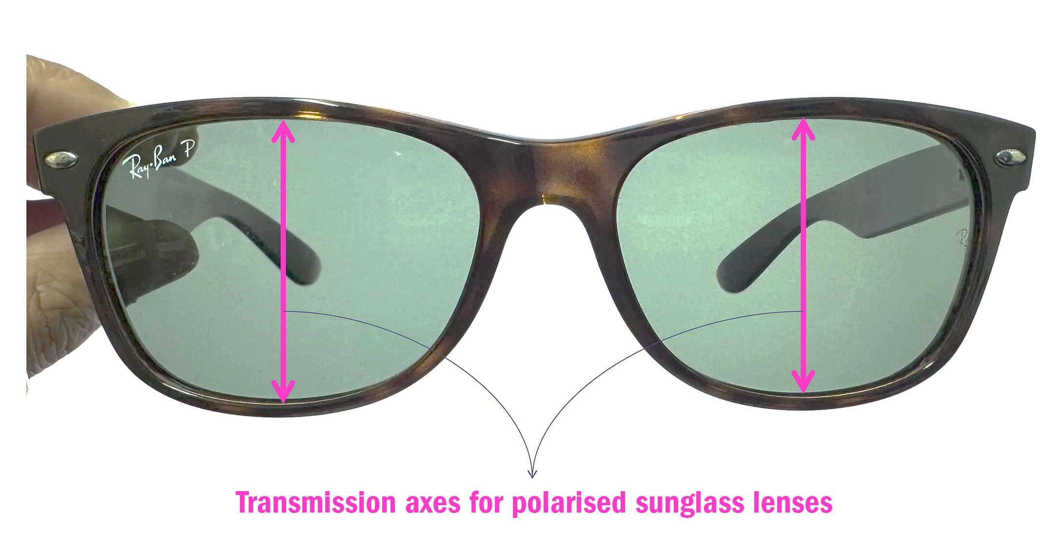
Figure 15a (taken without a lens, ie as observed by the viewer’s naked eye) suffers from significant reflective glare, which clearly obstructs the observer’s view of the underlying tarmac, leaves and other debris.
In contrast, these features are clearly visible at the bottom of/within the puddle in figure 15b, which was shot with a polarised sunglass lens in place.
Figure 14: A schematic depicting how polarised sunglass lenses are used to ‘absorb’ partially polarised light. The unpolarised incident sunlight (denoted by the five black double arrows) reflects off the water’s smooth surface and becomes partially polarised parallel to this surface (depicted by the green-coloured wave). As the transmission axes of the polarising sunglass lenses are orientated in the ‘vertical’ position, the lenses ‘absorb’ this polarised light, thereby stopping it from reaching the observer’s eyes. θi: angle of incidence (degrees), and θr: angle of reflection (degrees). The black dashed line represents the normal line formed at the surface
A critical comparison of these two photographic images highlights a significant reduction in reflective glare, and a corresponding substantial improvement in image clarity gained by simply wearing a polarised sunglass lens.
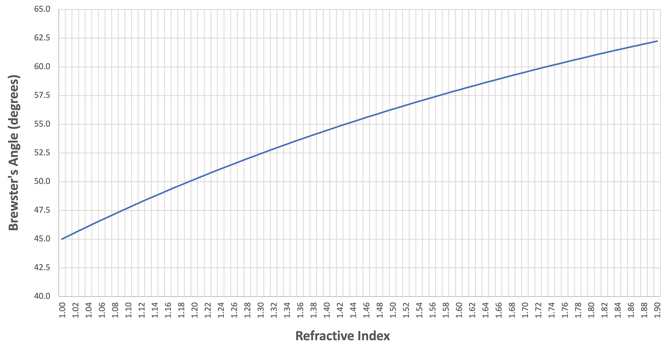
Finally, figure 16 presents a plot of Brewster’s angle (θB) as a function of the reflective material’s refractive index (n2). This graph illustrates that the magnitude of Brewster’s angle is relatively similar for a range of different liquids whose refractive indices typically range between 1.33 (where θB = 53.06 degrees) to 1.48 (where θB = 55.95 degrees).
Figure 15: Two photographic images (both captured using an iPhone 15 pro) providing a direct comparison of the degree of reflective glare observed off the surface of a large puddle of water on a bright day
15A (top): This image was shot without a polarised sunglass lens in situ and displays the high degree of reflective glare that would be seen by an observer’s naked eye.
15B (bottom): This image was shot with a polarised sunglass lens in situ, allowing the observer to comfortably view the underlying tarmac, leaves and other debris, which are clearly visible at the bottom of/within the puddle – highlighted via the red circles and white text
Furthermore, research shows that the refractive index of ice varies between 1.29 to 1.31,16 depending on the temperature in which the measurements were made. This range of refractive index values would yield Brewster’s angle values of 52.22 to 52.64 degrees, respectively.
This key information confirms that polarised sunglass lenses are also extremely useful for reducing solar reflective glare from ice and snow.
Figure 16: A plot of Brewster’s angle (θB) as a function of the reflective material’s refractive index (n2). In calculating these Brewster’s angle values (via Equation 3), it was assumed that the n1 value was 1.00, ie the reflective material in question was surrounded by air
Summary
This article summarised the early theories that postulated what light was and how it behaved when interacting with physical matter. The concepts of EMR and polarisation were introduced and discussed. A detailed overview of the structure and composition of a linear polariser (polarising filter) was provided.
Explanations of how both unpolarised and (either partially or plane) polarised light can be simply characterised, via decomposition into two orthogonal E field components, were presented. The key concept of polarisation induced through reflection at the surface boundary between water and air was then introduced and explained in detail. Readers were reminded that, rather than simply considering reflection in relation to the surface boundary, Fresnel’s equations specifically calculate reflectance for light polarised via reflection with respect to the POI.
Correspondingly, calculations were presented to highlight the significant difference in magnitude between the reflectance values for waves polarised perpendicular to and parallel to the POI.
A series of figures were also presented, including a graphical plot of how reflectance varies as a function of the angle of incidence and a plot of how the value of Brewster’s angle varies as a function of refractive index.
Additionally, a series of photographic images were also presented to provide cogent evidence of how a polarising sunglass lens significantly reduces reflective glare to improve visual clarity.
Overall, the scientific information presented within this article strongly supports the clinical recommendation of polarised sunglass lenses for drivers, cyclists, anglers and sailors who may complain about reflective glare off the surface of water.
Equally, polarised sunglass lenses will also significantly reduce solar reflective glare off ice and snow, making them an ideal choice for skiers and snowboarders too.
It is envisaged that the information presented in this article will prove useful for supporting ECPs in answering technical queries from well-informed patients who are keen to learn about why polarised sunglass lenses are the best option for them.
- Dr Amit N. Jinabhai is a qualified optometrist with a proven track record of excellence in optometric education and research. He is the founder of Jinabhai Regulatory Consultancy and currently works as a freelance consultant and locum. He has significant experience in the areas of regulatory decision-making and clinical auditing.
References
- Malus E-L. On the property of reflected light [Sur une Propriete de la Lumiere Reflechie]. In: Memoirs of Physics and Chemistry of the Arcueil Society [Memoires de Physique et de Chimie de la Société d’Arcueil]. Paris: Printing house of HL Perronneau, 1809. pp. 143-58.
- Land EH, inventor Polarizing Refractive Bodies. United States Patent Office (US1918848) 1933 (Filed 26 April 1929).
- Sliney DH. What is light? The visible spectrum and beyond. Eye. 2016;30(2):222-9.
- Newton I. Opticks: A Treatise of the Reflections, Refractions, Inflections and Colors of Light. First ed. London: Printed for Sam Smith and Benj. Walford; 1704.
- Descartes R. Discourse on the method [Discours de la methode]. Leiden: From the printing house of Ian Maire, in Leiden; 1637.
- Huygens CHDZ. Treatise on Light [Traité de la lumière]. Leiden: Pierre vander A (Bookseller); 1690.
- Young TI. The Bakerian Lecture. Experiments and calculations relative to physical optics. Philosophical Transactions of the Royal Society of London. 1804;94:1-16.
- Einstein A. On a heuristic point of view concerning the production and transformation of light [Über einen die Erzeugung und Verwandlung des Lichtes betreffenden heuristischen Gesichtspunkt]. Annalen der Physik. 1905;322(6):132-48.
- Lewis GN. The Conservation of Photons. Nature. 1926;118(2981):874-5.
- Smartt RN, Steel WH. Birefringence of Quartz and Calcite. J Opt Soc Am. 1959;49(7):710-2.
- Raman CV, Krishnan KS. Polarisation of Scattered Light-quanta. Nature. 1928;122(3066):169.
- De Senarmont H, Verdet E, Fresnel L. The Complete Works by Augustin Fresnel [Oeuvres Completes D’Augustin Fresnel] Paris: Imperial Printing (care of the Minister of Public Education); 1868.
- Tunnacliffe AH, Hirst JG. Light waves. In: Optics Second ed. Kent, UK: The Association of British Dispensing Opticians, College of Education, 2002. pp. 291-310.
- Langenbucher A. Law of Refraction (Snell’s Law). In: Encyclopedia of Ophthalmology (Schmidt-Erfurth U, Kohnen T, editors): Springer, Berlin, Germany, 2018. pp. 1042.
- Brewster D. IX. On the laws which regulate the polarisation of light by reflexion from transparent bodies (in a letter addressed to Right Hon. Sir Joseph Banks). Phil Trans R Soc. 1815;105:125-59.
- Rocha WRM, Rachid MG, McClure MK, JH, Linnartz H. Water ice: Temperature-dependent refractive indexes and their astrophysical implications. Astronomy and Astrophysics. 2024;681:A9.1-A9.12.