Domains and learning outcomes (C111067)
• One distance learning CPD point for optometrists and dispensing opticians.
• Clinical practice
Upon completion of this CPD, ECPs will be able to list the different types of scanning protocols available for OCT imaging (s5)
Upon completion of this CPD, ECPs will be able to describe the different types of maps and charts generated by OCT imaging (s5)
In the first article in the series, we briefly refreshed our knowledge of retinal anatomy and introduced ourselves to basic concepts and terminologies in optical coherence tomography (OCT).
In this second article, we will explore the data is extracted from these scans and how this data is represented to clinicians. We will also explore how to differentiate layers and lesions on B-Scans and different ways to view OCT B-Scans and other forms of OCT imaging, like OCT-A, OCT Topography and biometry, for example.
Understanding Scan Types
Most OCTs capture scans in several ways. As mentioned in article 1, a cross-sectional scan is known as a B-Scan. A single B-Scan can be captured rapidly with OCT; this represents a single ‘line’ scan across one single part of the posterior pole.1, 2
Such a scan can only show any pathology present along the direction of that line. A line scan can be horizontal, vertical or along any diagonal angle. Usually, scan lengths range from 3mm to 12mm on most devices, although some go out to 21-22mm.
To obtain more information about the macula, or disc, for example, it is a good idea to take multiple scans across an area. Such scans may be composed of roughly 10 to 12 B-scans, either in a clock face pattern, or in a small grid, for example.
Volumetric scans, also referred to as 3D cube, mesh or map scans, can also be useful. Volumetric scans are usually comprised of 64, 128 or 256 B-Scans, rapidly captured, at lower resolution from the top to the bottom or the left to the right (for example) of the scan area. The advantage of this scan type is that measurements of layers and the total retina can be taken on each B-Scan and then an understanding of the retinal tomography and morphology can be ‘mapped’. Measurements can be represented graphically and can also be compared to normative data for improved diagnostic purposes. Where multiple line scans are used, this is also termed a raster scan, comprised of raster lines.3
Circular scans around the optic nerve head can also be captured and used to measure RNFL (retinal nerve fibre layer) thickness and, again, this can be compared to normative data too.4
Figure 1, below, shows an image I used to use in OCT lectures about 10 years ago representing the scan options found on the Nidek RS-330 OCT. These scans are commonly found on most OCTs in one form or another.
The various scan protocols can be altered in size, area and position on the retina/posterior pole and optic nerve head.
Some of these scans contain more data, allowing for numerous maps and charts to help understand more about retinal or optic nerve dimensions, morphology and how these compare to ‘normal’ values.
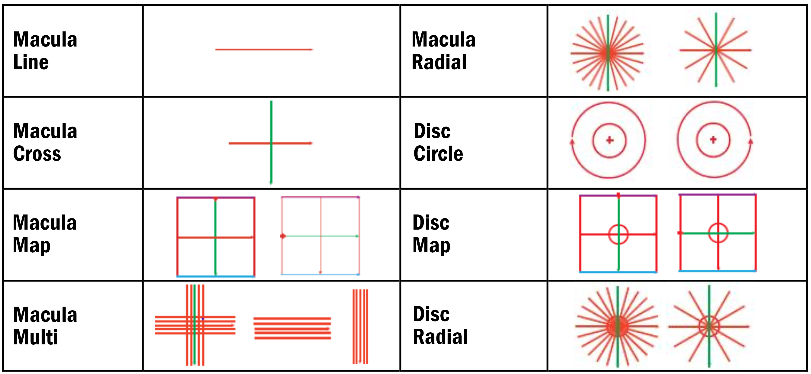
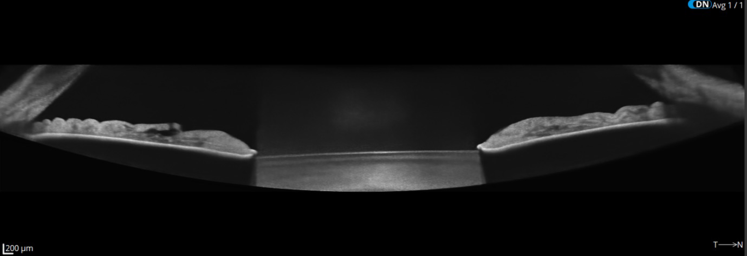
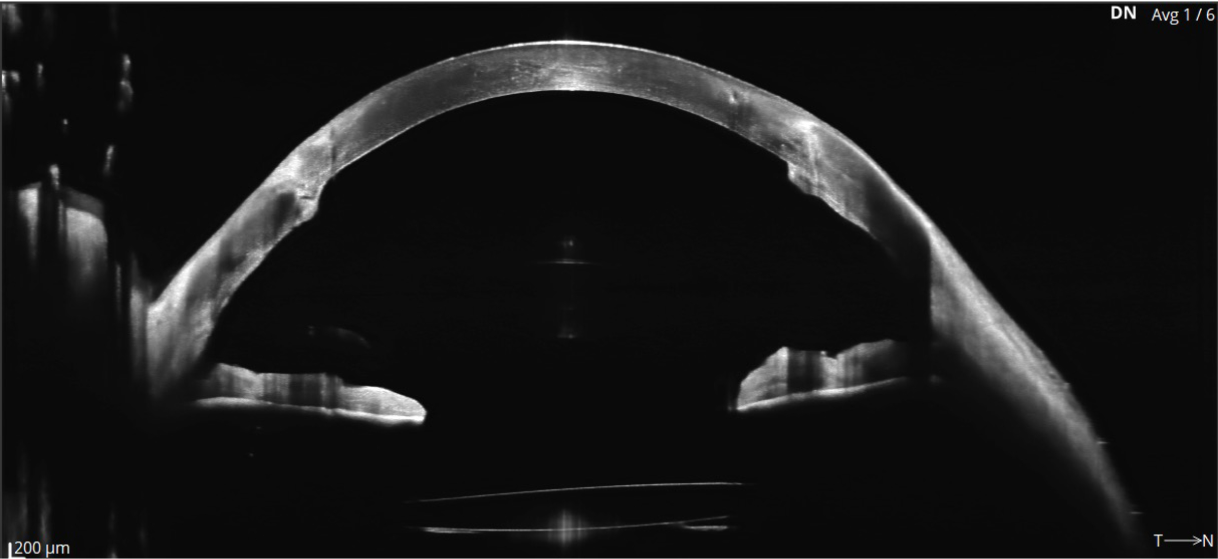
Most OCTs can also capture anterior eye scans, primarily of the cornea and anterior chamber angle. Some OCTs can capture full ‘angle to angle’ scans, and, in some cases, full anterior chamber scans and even scleral scans. More modern OCTs may also provide topography and tomography maps and data for the whole anterior segment (AS-OCT).5
The three images for figure 2 shows some examples of anterior scans that are available from several OCTs. Figure 2a (top) depicts ‘Angle to angle’ B-Scan from the Optopol Revo FC OCT showing Iris and anterior lens, while in figure 2b (middle) the wide scan shows an IOL in place and penetrating keratoplasty (Revo OCT). Lastly, figure 2c has a Cylite HP OCT image of a 3D anterior segment scan showing a scleral lens in place and clearance measurements shown across a map of corneal topography (clearly a keratoconus patient).
Understanding Retinal B-Scans
In the first article, we examined some basic details of the B-Scan. We will now look more closely at reflectivity and shadows.
When examining B-Scans, it is important to consider reflectivity and shadows to differentiate layers, fluid, lesions and other features.
Reflectivity
Some layers and lesions are more Hyper-Reflective (brighter):
- EZ (ellipsoid zone) and RPE Bruch’s complex
- RNFL, ELM and ILM
- Hyaloid face
- Epi retinal membrane (ERM)
- CNVM (choroidal neovascular membranes) and scarring
- Blood and exudate
- Pigment clumps
See figure 3 to see examples.
Some layers and lesions are more Hypo-Reflective (darker):
- Outer and inner nuclear layers.
- Vitreous
- IZ and MZ (interdigitation zone and myoid zone)
- Serous fluid
- Shadows (some people like to suggest shadows are hypo-reflective, but they are caused by the signal being totally blocked by what is inner to/above the area in shadow).
Figure 3a and b: Examples of hyper reflectivity on OCT B-Scans. Notice the shadows beneath the exudate and blood
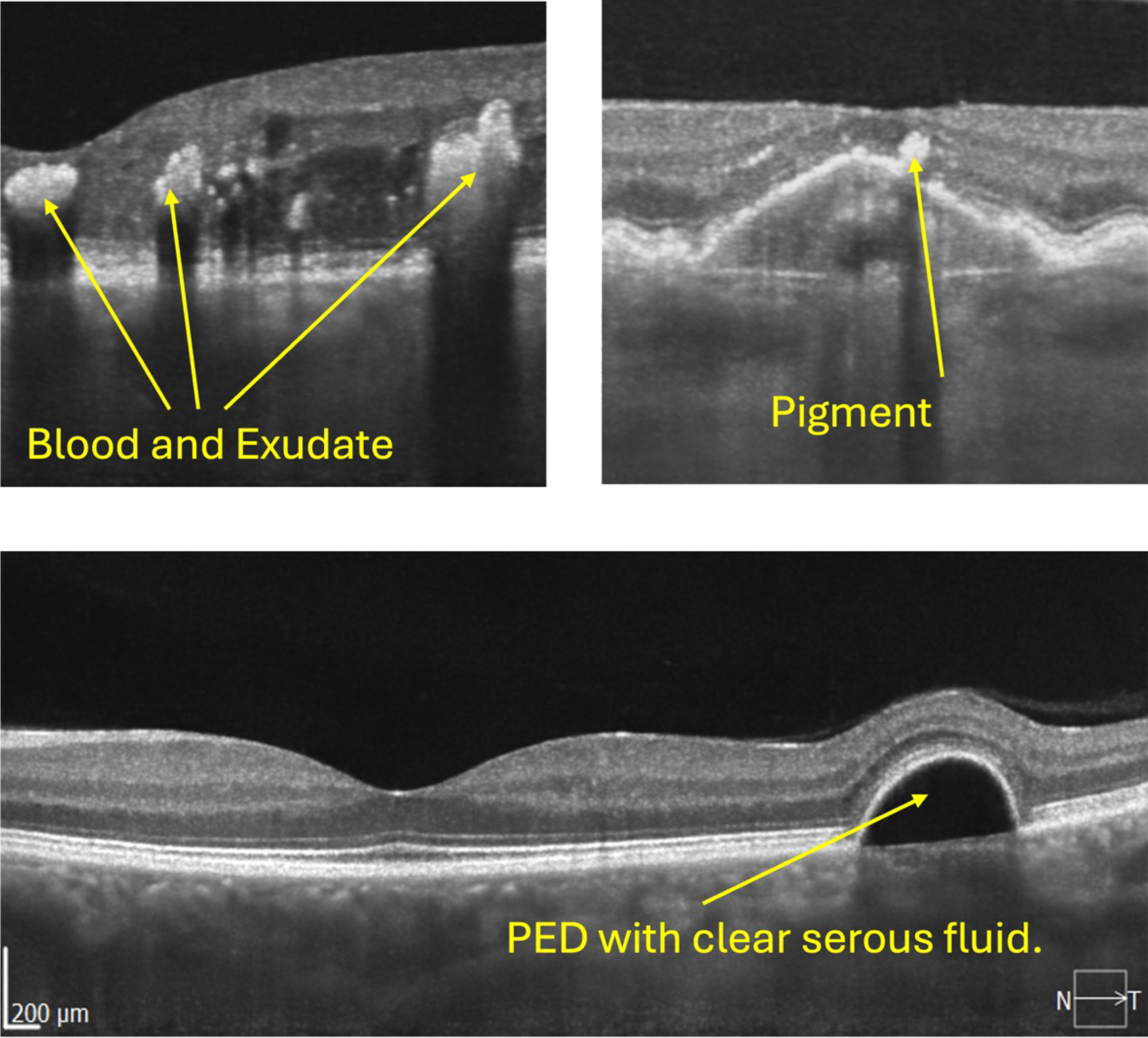
Figure 3c: Note, there is no shadow beneath the serous fluid and Bruch’s Membrane can just be seen
If we look at figure 3c, we can see a PED (pigment epithelial detachment), where the whole retina, including RPE is lifted away from Bruch’s membrane and, therefore, lifted away from the choroid. The clear (serous) fluid underneath is also known as sub-RPE fluid (not SRF – sub retinal fluid).
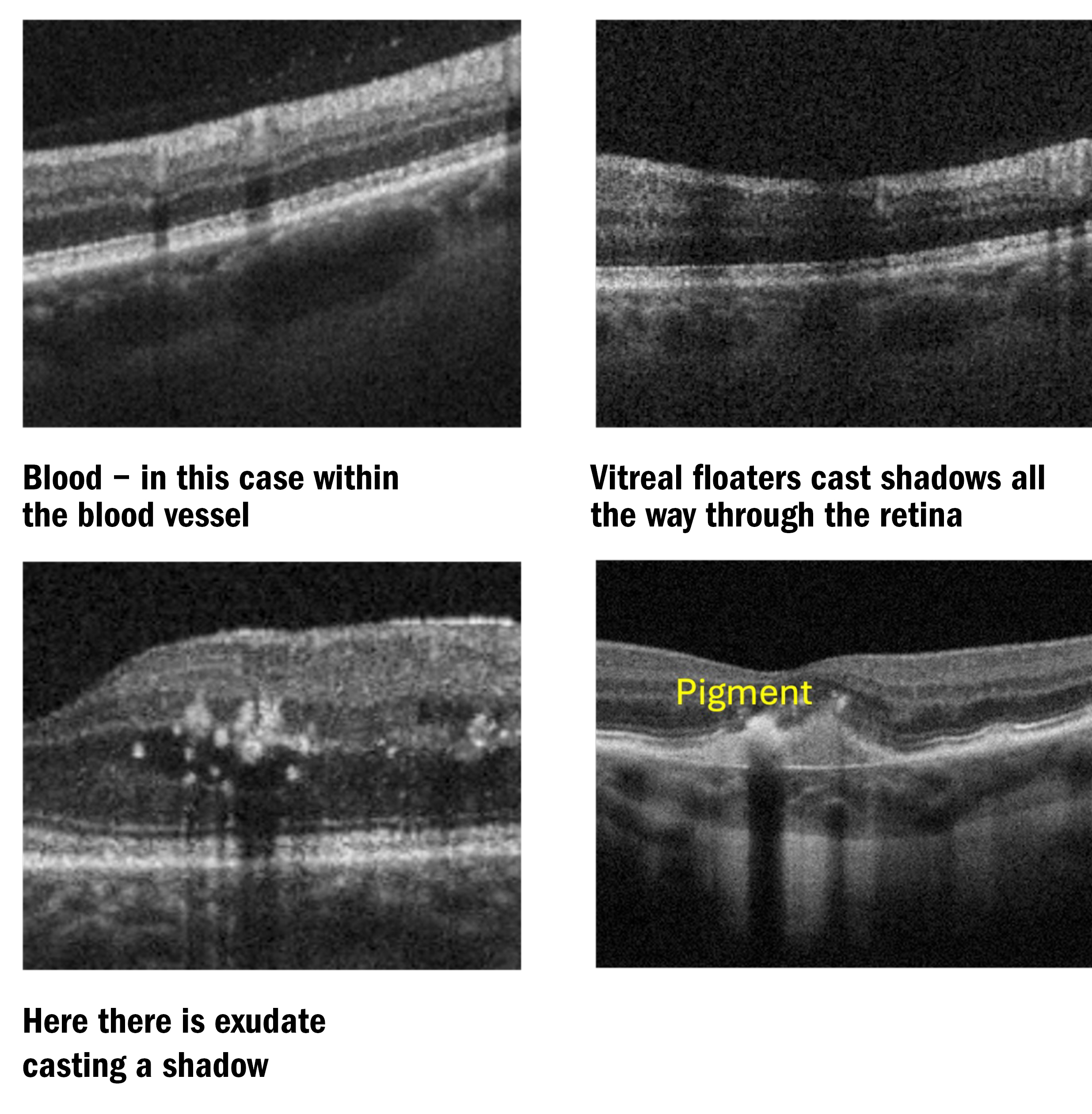
Another feature to be aware of when evaluating B-Scans is shadows. Shadows are to be expected in healthy eyes from blood vessels, for example, but they can also indicate the presence of pathology. Blood, exudate, media opacities (including vitreal floaters) and pigment clumps can all cast shadows (see figure 4).
Another common sign on B-Scans is ‘reverse shadowing’, also known as ‘window defect’. This usually occurs where the RPE is absent or misplaced, so more of the infrared laser signal can reach the choroidal layers and ‘illuminate’ them more intensely.6
Figure 5 shows examples of window defects commonly found on OCT B-Scans. GA (geographic atrophy) will often lead to large and dramatic areas of reverse shadowing. A colleague of mine suggested these defects look like a ‘waterfall in the choroid’. I think this is an excellent analogy.
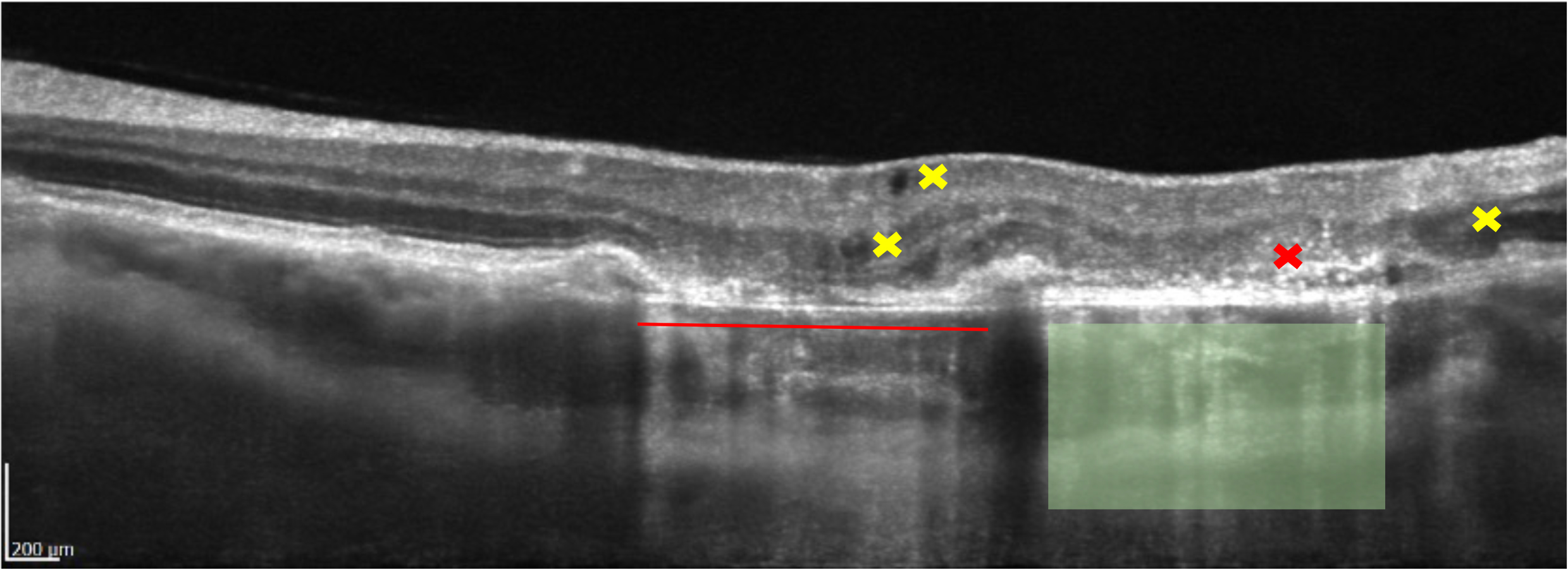
You will notice on figure 5 some dark areas within and between the retinal layers. Dark voids can be observed next to the yellow crosses l; these are hypo-reflective and do not cast shadows, they represent clear, serous fluid. As the dark areas are within or between the retinal layers, these lesions are known as IRF (intra retinal fluid) or intra retinal cysts. We can see that the areas are rounded, this means they are more likely due to fluid leakage as opposed to voids created by traction.7
Next to the red cross, many white dots/spots can be observed, these are known as intra retinal HRF (hyper-reflective foci). In this case, pigment clumps being released from the dying RPE8 (retinal pigment epithelial) cells and from ‘emptying’ drusen. However, the spots could also represent:
- Lipids or Muller cell debris – particularly in diabetic eye disease and AMD (age-related macular degeneration). The spots could also be signs of activated microglial cells, which are immune cells from the inflammatory response.
- Signs of ischaemia, such as retinal vein occlusion.
HRF tend to represent more severe outer retinal atrophy and a poorer prognosis for visual outcomes in retinal disease, particularly AMD and DMO (diabetic macular oedema).9
Maps and normative data
To gain more information more rapidly from scans, particularly volumetric scans, it is useful to graphically represent the data gathered from the scans, such as total retinal thickness, individual layer thickness, thickness of the GCC (ganglion cell complex), RNFL thickness, comparison to normative data, for example. Such information is useful to quickly spot signs of a range of ocular diseases, including glaucoma.
It is important, however, to understand the limitations of OCT normative data with reference to glaucoma.10 We will see in a future article how many false positive referrals come about because of the incorrect application of OCT normative data and glaucoma ‘suspects’ in particular.
For this article, examples from the Nidek RS-330 OCT and the Optopol Revo OCT are used.
The Macula Map Scan overview, on the Nidek RS-330, contains several sections, which can be highly informative regarding the patients’ ocular health.
In figure 6, we can see a range of maps and charts that appear colourful, but are perhaps a little confusing to newcomers to OCT.
This is a normal example of a LE scan. You will notice that the left-hand side of the macula map shows total macula information, and the right-hand side of the macula map shows information relating specifically to glaucoma.
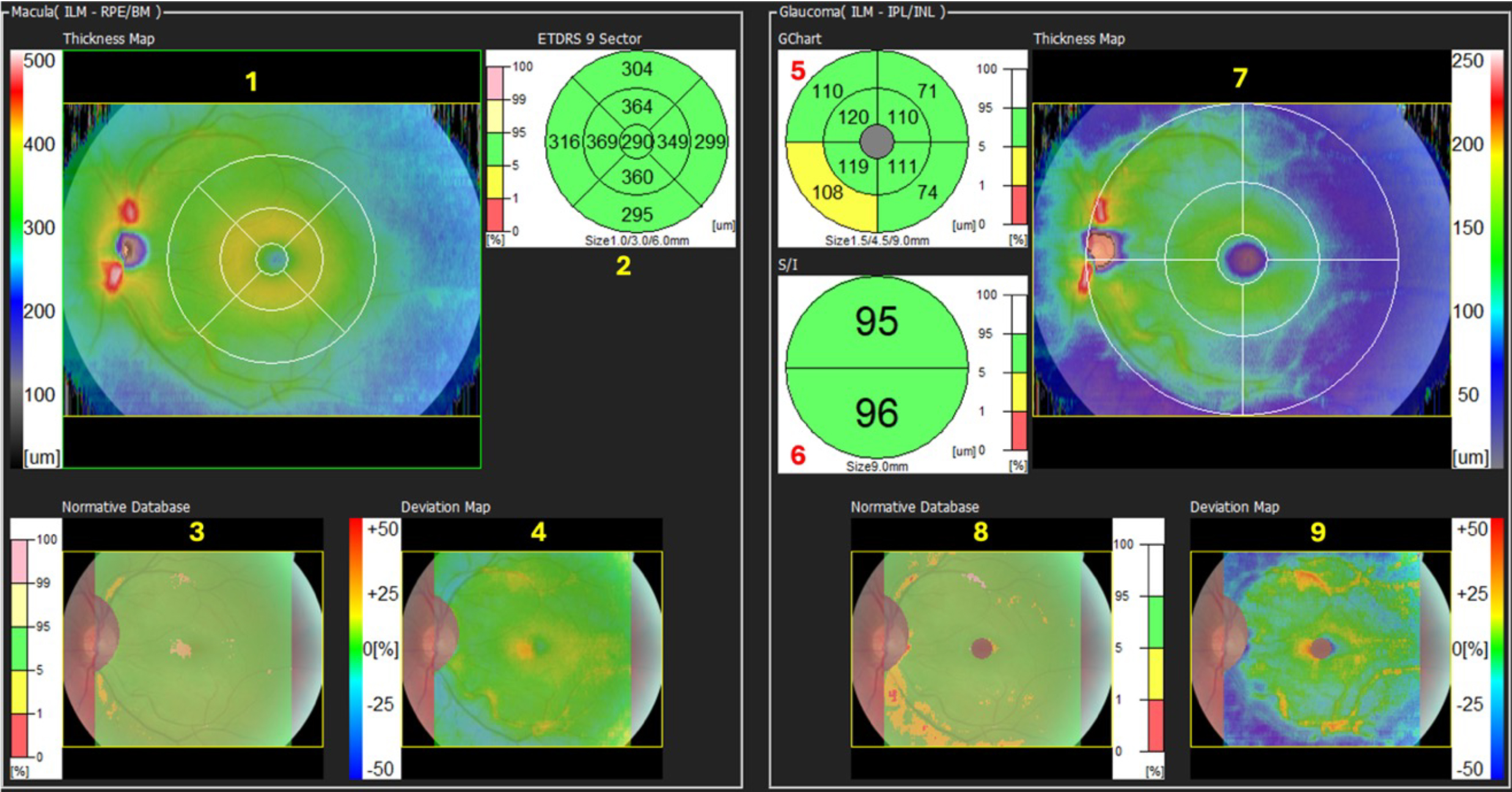
Viewing the numbers in figure 6, we can see as follows:
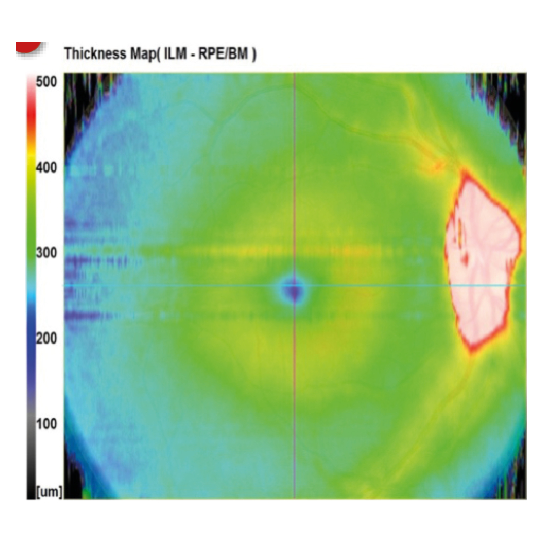
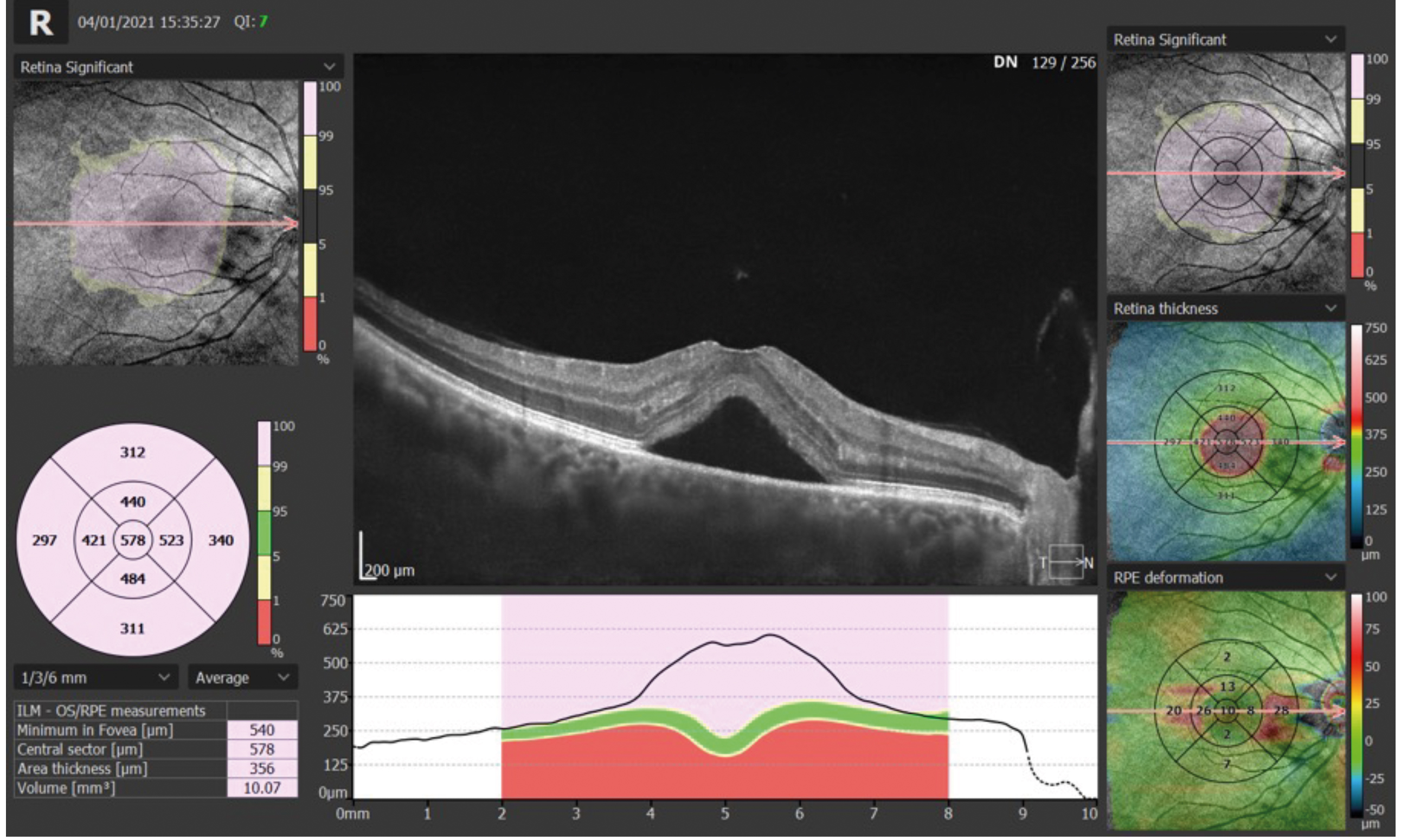
1. The Thickness Map.
In this case, it refers to the total retinal thickness within the boxed area. In this example, it is a 12mm H, by 9mm V box centred on the fovea. The colours represent retinal thickness in microns and relate to the scale at the side of the map.
That scale ranges from 0 to 500 microns, thicker than this is represented by white. The dark grey and blue colours show thinner areas, the green colours represent thicker average retinal values, and the yellow/red colours represent even thicker areas.
I have heard many ways of describing these maps, but my favourite description is to consider the map like a geographical map. Imagine the blue is the sea, it is lower/thinner. The green is the land, it is green and higher, lighter green areas are higher ‘foothills’. Orange and red areas represent higher hills and smaller mountains and thicker areas. Where there is white on the map, this represents the ‘snow-capped peaks’, the highest and thickest parts of the map.
In figure 7a, we can see a normal thickness map:
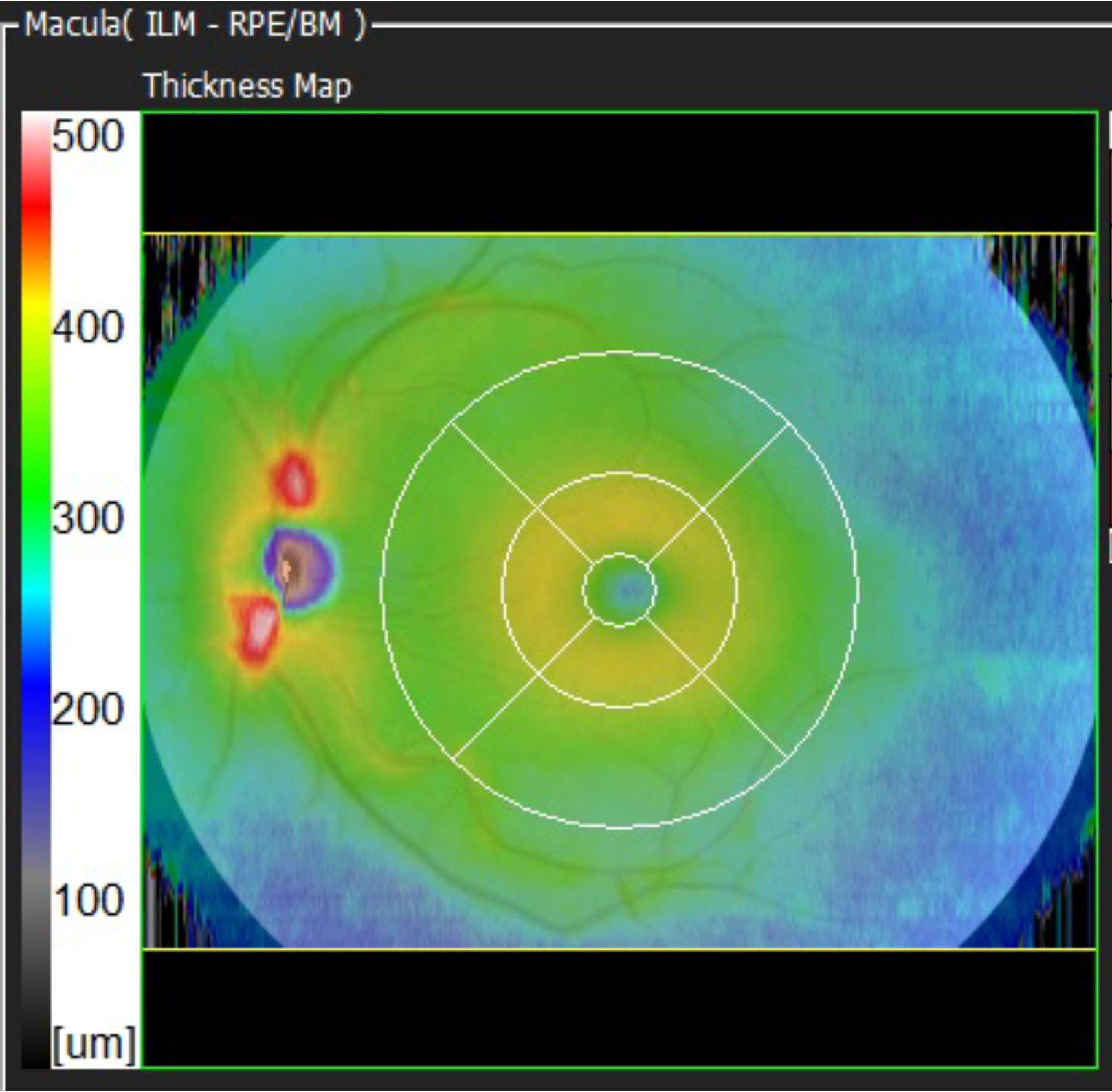
We have snow-capped peaks superior and inferior to the optic nerve head in most cases and a raised area around the fovea – the parafoveal area. The thinner peripheral retina is blue and is lower (the sea).
If we look at some example pathologies, we can understand a lot from the thickness maps alone.
Looking at Figure 7b, we can see a white rounded area centrally. This represents an area that is thicker than 500 microns. This is not normal, of course, for the central retina on a thickness map. But what could it be? The two main explanations would be oedema causing thickening, or traction causing vertical ‘stretching’ or lifting of the retina. In this case, look at the shape of the lesion. It is round and regular. Almost invariably, this means that fluid is causing the lifting.11 From the thickness map alone, we cannot be sure if the fluid is serous, sero-sanguinous (turbid) or is blood. We will discuss the nature of fluid in more detail in a later article. In this case, it was serous fluid and was caused by CSR (central serous retinopathy).
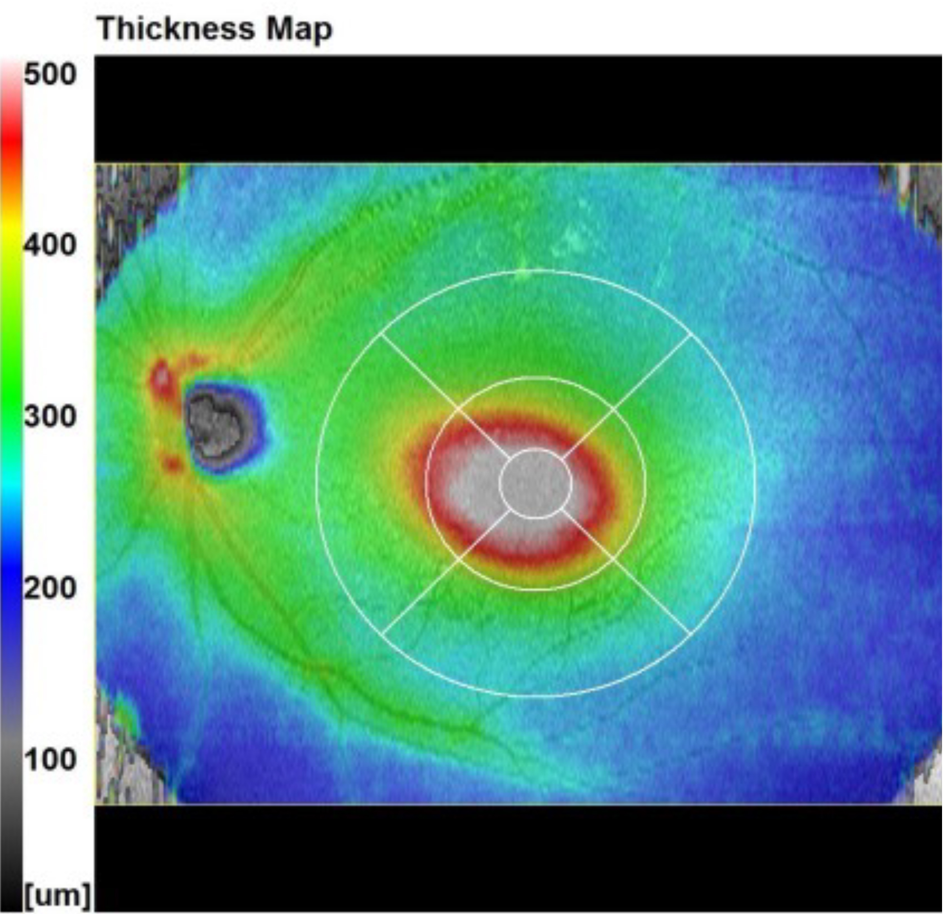
Figure 7c, below, however, shows central lifting, which is irregular and angular. This is much more likely to be tractional lifting such as from an ERM (epi retinal membrane) or VMT (vitreo macular traction), for example. This case was caused by a significant fibrous ERM.11
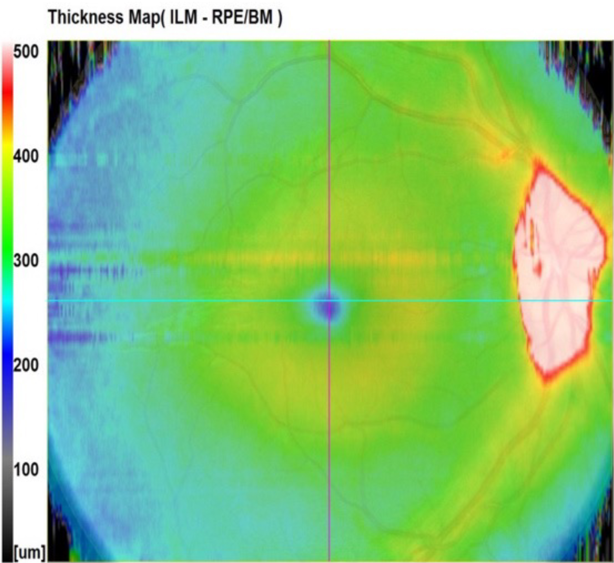
Figure 7d appears normal at first glance. However, if you look at the optic nerve head and surrounding tissue, you can see that the whole area is white (off the thickness scale). This is not normal and could represent a pathological raised disc or buried disc drusen, for example.12 In this case, it was papilloedema that led to this raised area.
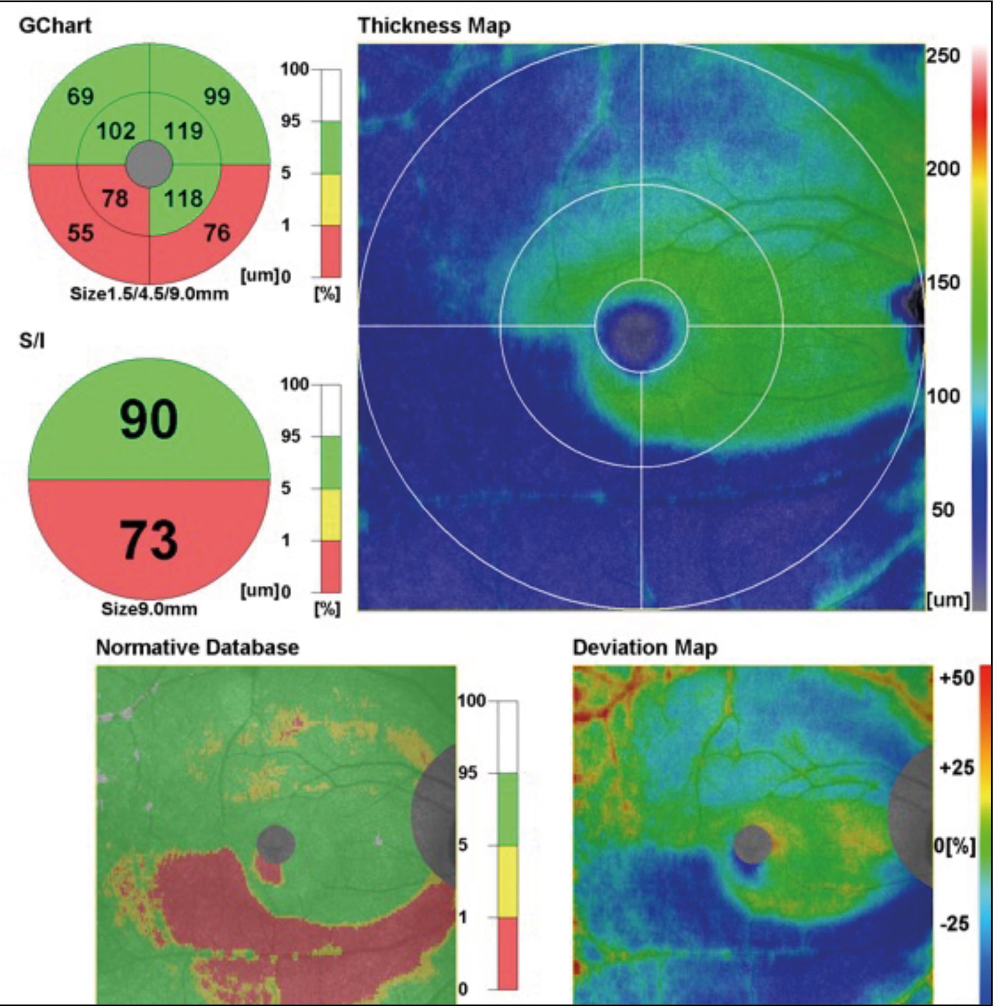
2. The ETDRS Map.
This chart is a normative display of the central 6mm zone of the macula centred on the fovea. You can see an overlay of it on the thickness map too.
The ETDRS (Early Treatment Diabetic Retinopathy Study) grid or map was devised in the 1980s by the NEI (National Eye Institute) in the USA as part of a multi-site study that required normalisation of data collection.13 It was not designed for OCT, but it has been used by OCT manufacturers as an internationally recognised normative map of the central retina.
Each of the nine sections on the OCT ETDRS shows a number that represents the average total retinal thickness within that section. That figure is compared to a normative database (NDB). The patient’s age, sex and ethnicity are required to compare to the patient to the correct cohort within the NDB.
The scale on the side is a percentage scale, representing the proportion of the normal population that has a retina of that average thickness in each section.
Imagine the scale represents a normal distribution. The green area represents the main 90% of the normal population and the other colours represent the first and second standard deviations thicker and thinner than the mean.
Figure 8 shows this representation graphically. The green colour simply suggests that this patient’s retina is roughly equal to the average thickness of around 90% of the normal population. It is not a traffic light system.14
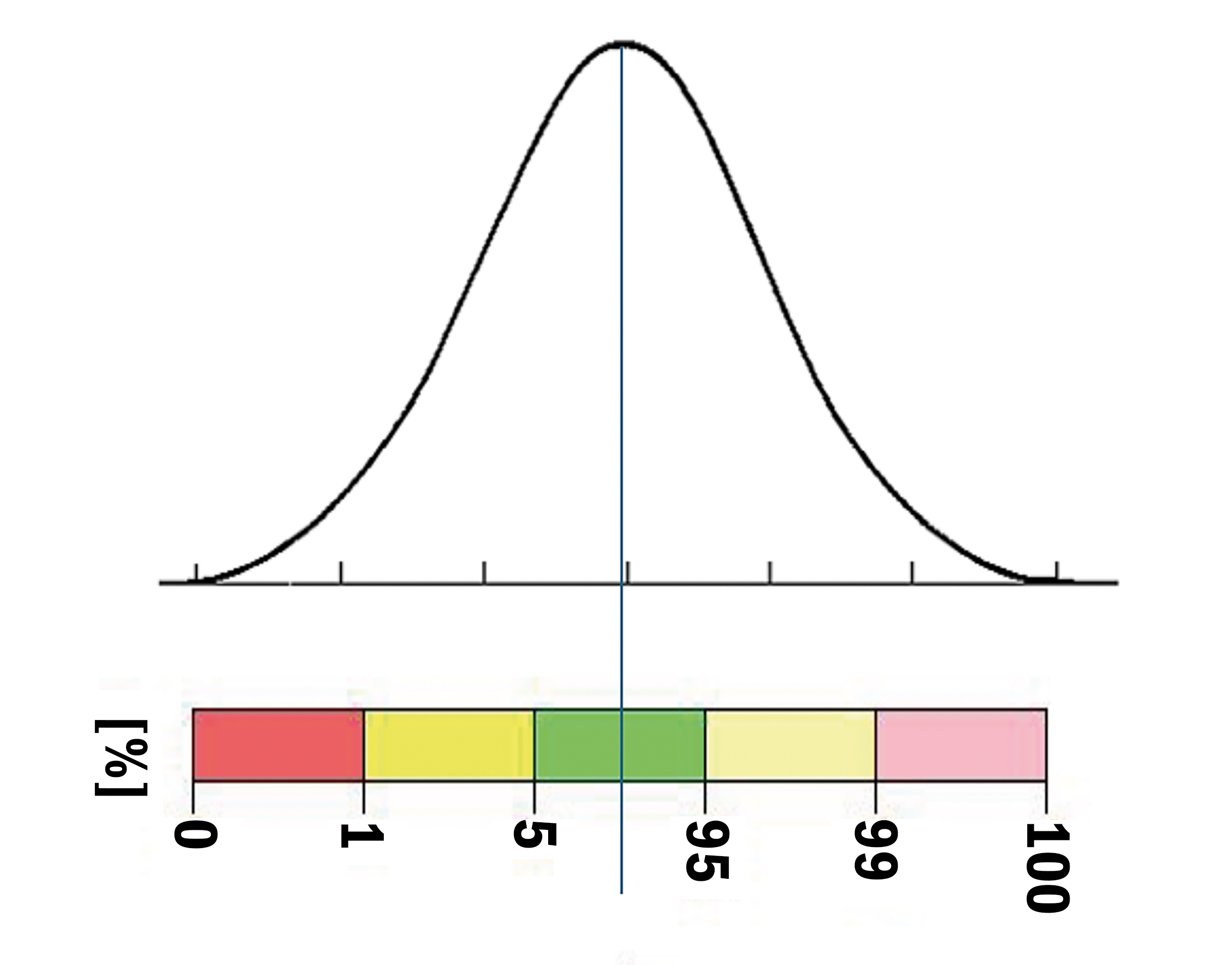
The red tells us that the patient’s retina is thin and equates to less than 1% of the normal population’s retinal thickness. The yellow represents a thin retina equating to between 1% and 5% of the normal population. Green equates to retinal thickness between 5% and 95% of the normal population. The pale yellow is thicker than the mean and equates to between 5% and 1% (shown at 95% to 99%) of the normal population and the pink is thicker still, equating to less than 1% (shown as 99% to 100%) of the normal population.
These colours are roughly the same on all OCTs and were invented many years ago by the original inventing team.15
Normative data plots are not designed to diagnose retinal conditions or glaucoma. The colours are perhaps not helpful as reds and yellows can be misconstrued as being emotive or sight threatening. This is not the case. I believe a significant number of referrals occur because red is considered ‘danger’ to many. Ophthalmologists even refer to these referrals as for ‘red disease’.16
As we will see in a later article, the normative databases do not contain many eyes or subjects and the range and mix of these is minimal and highly restricted by stringent exclusion criteria.17 This means the NDBs are usually too sensitive, but not specific enough, certainly for glaucoma. Most OCTs have sensitivity averaging around 94% and specificity around 95%, but the specificity is still too low for glaucoma.18
3. Normative Map.
This 9mm x 9mm plot represents the same normative data as in the ESCRS, but across the whole boxed area, not just within the 6mm circle.
4. Deviation Map.
This 9mm x 9mm plot shows, in percentage terms, how much thinner or thicker each point is compared to the NDB. The cool colours show % thinner and the warm colours show % thicker. Green suggests 0% difference in the patient’s retina compared to the NDB.
5. The G-Chart.
This is the first chart on the ‘glaucoma side’ of the macula map. It is a measure, in this case, of the RNLF, the GCL, IPL and INL boundary. This is considered the GCC (ganglion cell complex) and represents the only part of the retina affected by glaucoma. This is again compared with normal values referring to this patient’s NDB cohort. Therefore, if there is thinning of the GCC, particularly fitting an arcuate type of pattern, this could represent an increased risk of glaucoma.19
Again, the normative data on OCTs is not broad enough to be used in isolation as a strong diagnostic marker for glaucoma. It should be used as an indicator of potential higher risk. The key is to then compare the patient to themselves.20 In other words, if there is apparent risk, check for change over time and, if there is no progression, then there is no active disease. This chart covers a central 9mm circular area centred on the fovea.
6. The S/I Comparison Chart.
This is also part of the GCC chart but looks specifically at vertical asymmetry between the temporal GCC along the horizontal midline. Ultimately, this helps find early signs of glaucomatous change associated with the temporal horizontal raphe.21 So, if there is a considerable asymmetry between the upper and lower hemisphere, it could indicate a higher risk of glaucoma.
7. The GCC Thickness Map.
This is a map of the GCC thickness shown in microns. It can show signs of loss of GCC/RNFL. Looking at figure 9, below, we can see an example of a confirmed glaucoma patient, where we can see a nasal step and an arcuate loss.
8. The GCC Normative Data Map. This map covers the normative data used in the GCC chart, but over the full 9mm x 9mm boxed area.
9. The GCC Deviation Map.
This map simply shows in percentage terms how much thicker the patient’s GCC is compared to the corresponding normative data.
Figure 10a shows a scan from the Optopol OCT software. You can see many similarities compared to the Nidek software.
The example in figure 10a shows a case of CSR (central serous retinopathy). Note the RPE/Bruch’s complex is still in place. The neural retina, including photoreceptors, is lifted away. The hypo-reflective area beneath shows that this is clear, serous fluid. As it is below the neural retina, it is known as SRF (sub-retinal fluid).22
Now that we have looked at macula and retinal maps and normative data, we will take a final look at the disc and ONH (optic nerve head). Figure 11 shows a RE single ‘disc 3D’ scan from the Optopol Revo OCT. Again, I have labelled the image with numbers to identify key elements. Most of these can be found on disc scans on other OCTs.
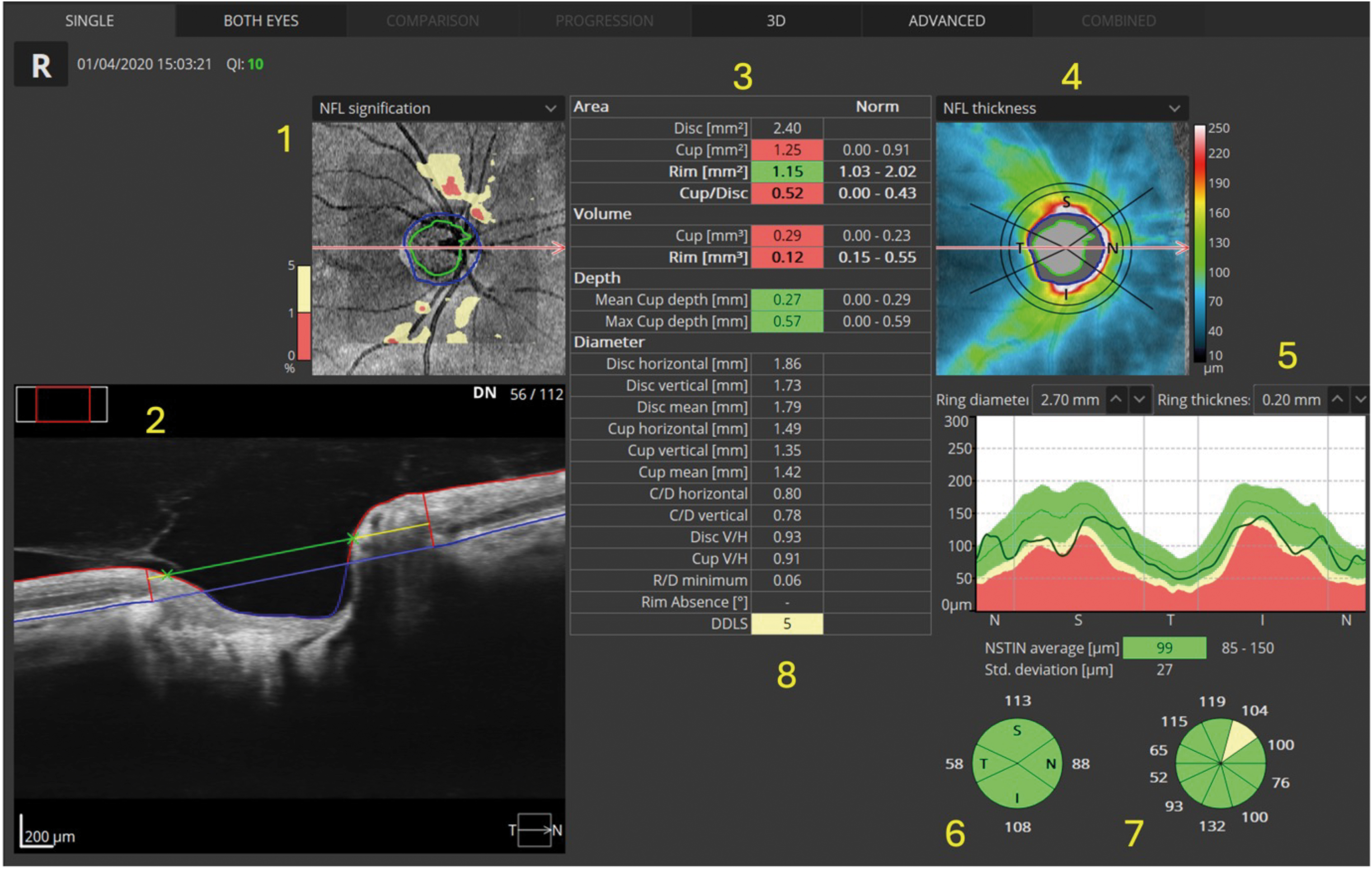
In this case, you may notice that the RNFL is thinner than the average for the normative data. It is imperative that all other diagnostic information available to you is considered. If there is no visual field loss, no obvious disc damage on fundoscopy, ‘normal’ intra ocular pressure and no other signs or symptoms, then this RNFL thinning may, in fact, be normal for this patient.
We may need to establish loss over time before considering this active glaucoma or other neuropathy, so monitoring may be considered, and, if undertaken, the same device should be consistently used.23
From the numbers in figure 11, above, we have the following:
- The normative thickness map for the RNFL around the optic nerve head. The pale yellow and red being the areas that are below the central 90% of the normal population. We are often only interested in thinning.24
- The ONH B-Scan. We can see the blue line represents Bruch’s membrane and the vertical red lines appear where the opening in Bruch’s membrane occurs (this delineates the disc margin to the OCT software).25 The green line represents the cup diameter estimation, and the yellow line is the disc diameter estimation; this is how the software calculates the CD ratio.
- Table of disc area, volume and depth, compared to ‘normal’ values on the right-hand side of the table. Where numbers are highlighted with red or yellow, the software is suggesting the figures are below or well below average. However, as previously mentioned, the ‘average’ comes from a narrow band of ‘ultra normals’ and may not represent reality.
- Thickness map of RNFL, the cooler colours being thinner and the warmer colours being thicker. White areas mean the RNFL in that area is ‘off the scale’ and are thicker than the scale measures.
- This is the NSTIN (or TSNIT depending on the software or settings) and is a very important chart; it is created from a circular scan roughly 3.4mm in circumference around the disc.26 The chart shows a flat two-dimensional representation of this circular image ‘unfolded’ onto the screen. We see the dark line showing the patient’s RNFL thickness around the nasal, superior, temporal, inferior and back around to the nasal part of the disc (hence TSNIT). As expected, the thickest parts of the RNFL will be superior and inferior (due to the nerve fibre bundles) and, according to the ISNT rule, the thinnest part of the RNFL should correspond with the temporal disc.
Figure 11a shows the NSTIN in more detail. The colours show the mean and thinner first and second standard deviations in yellow and red. In this case, the superior nerve fibre layer is just about ‘dipping into the red’, suggesting loss. However, this patient may naturally be like this and may not have changed much in decades, for example.27
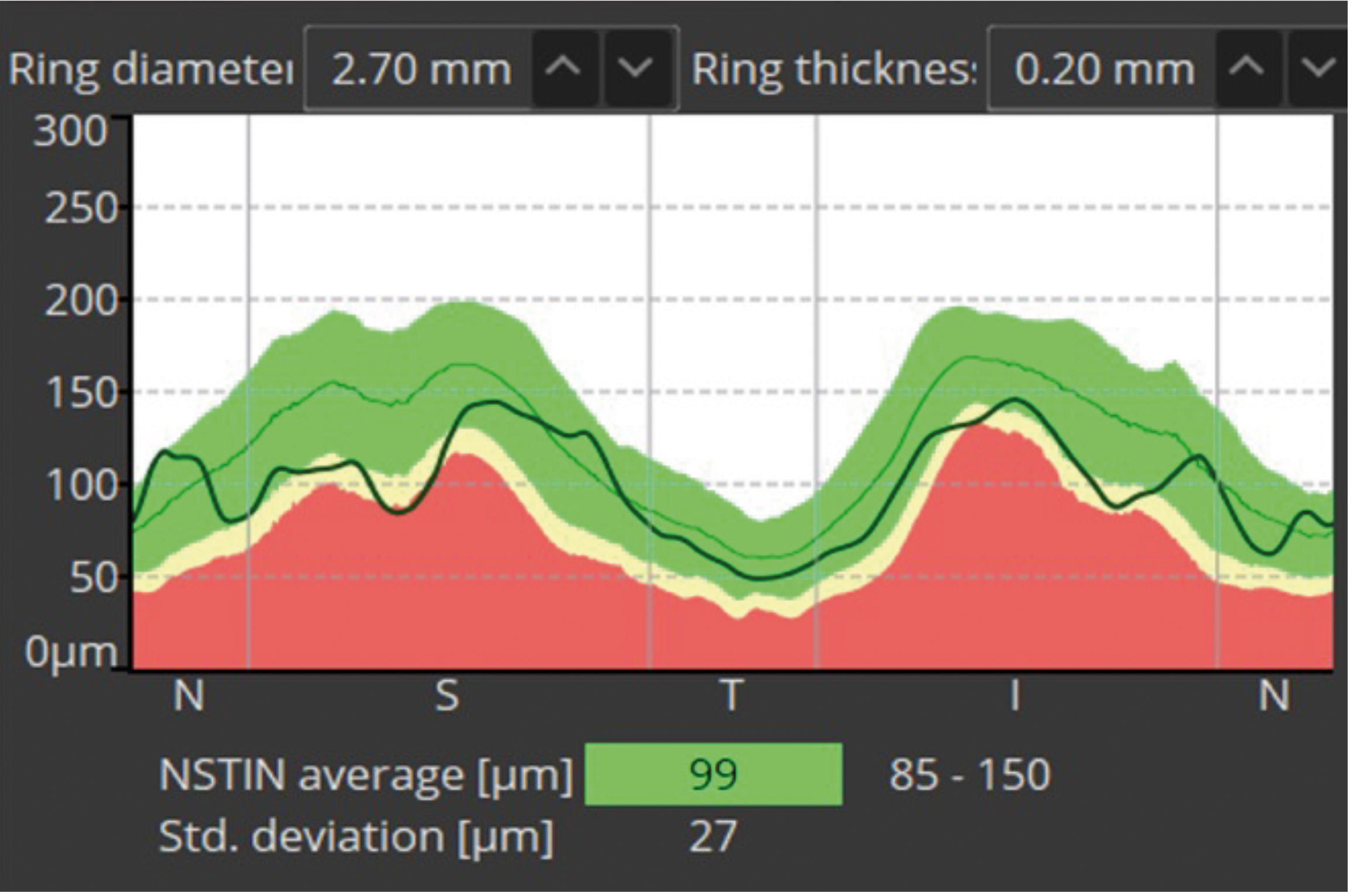
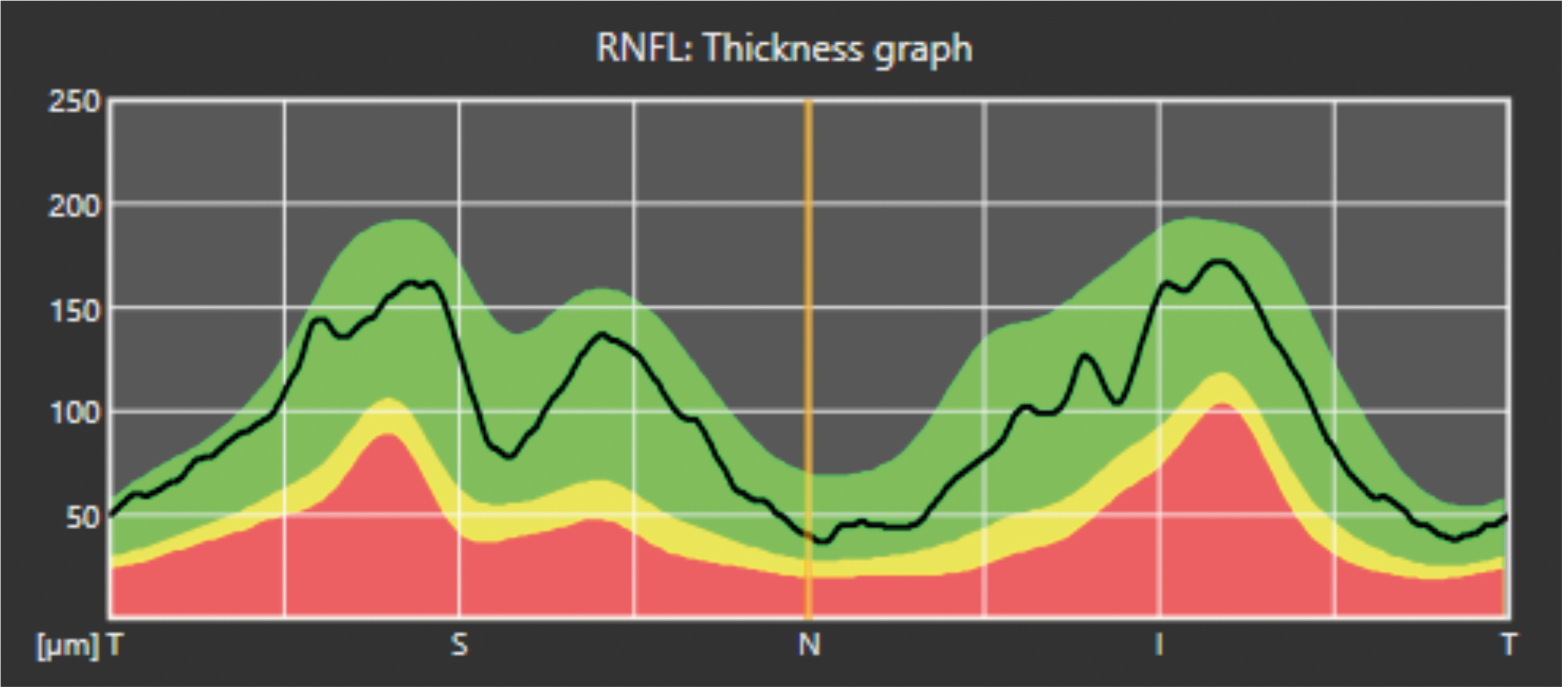
Figure 11b shows another example of such a display, from the Nidek RS-330. In this instance, we have a TSNIT diagram, starting at the temporal disc.
The chart in Figure 11b shows a ‘healthy’ disc, all green, suggesting the RNFL for this patient is equivalent to roughly 90% of the normal population for their age, sex and ethnic cohort. As we will see in a later article, it is not as simple as this.
6. ISNT rule represented graphically. Without going into too much detail, there is evidence that Black and Hispanic populations may have much greater visual field loss than the ISNT rule would suggest.28 However, for a quick understanding of ONH morphology, this is still a useful chart.
7. ‘Clock face’ diagram of the disc/optic nerve head. It helps to define areas of notching of the disc,29 and this may also define the position of Beta PPA (peri papillary atrophy),30 which often coincides with notching and can represent areas of significant RNFL loss and an increased likelihood of glaucoma being present. RNFL loss most commonly commences supra and infra temporally.31
8. Table shows data for different diameters, such as horizontal and vertical cup and disc, for example. In glaucoma, we often find the vertical CD ratio is larger than horizontal, for example. You will also see the DDLS (Disc Damage Likelihood Score), which is based on research by Spaeth et al.32 It is an attempt to better understand the morphology of the optic nerve head and its relation to glaucoma risk. However, it was not designed originally for OCT. Other OCTs, like those from Topcon, for example, also use the Hood report, which has been shown to be useful in diagnosing glaucoma more effectively with OCT.33
- Jason Higginbotham is an optometrist and dispensing optician with 35 years’ experience in the field.
- In the next article, we will look at B-Scans more closely, considering the most common lesions with some example cases.
References
- Bussel, I, Wollstein, G, & Schuman, J. (2013). OCT for glaucoma diagnosis, screening and detection of glaucoma progression. The British Journal of Ophthalmology, 98, ii15 - ii19.
- Cheong, H, Devalla, S, Chuangsuwanich, T, Tun, T, Wang, X, Aung, T, Schmetterer, L, Buist, M, Boote, C, Thi’ery, A, & Girard, M. (2020). OCT-GAN: Single Step Shadow and Noise Removal from Optical Coherence Tomography Images of the Human Optic Nerve Head. Biomedical optics express, 12 3, 1482-1498Ahlers, C, & Schmidt-Erfurth, U. (2009). Three-dimensional high resolution OCT imaging of macular pathology. Optics express, 17 5, 4037-45.
- Schuman, J, Pedut-Kloizman, T, Hertzmark, E, Hee, M, Wilkins, J, Coker, J, Puliafito, C, James, G, F, & Swanson, E. (1996). Reproducibility of nerve fiber layer thickness measurements using optical coherence tomography. Ophthalmology, 103 11, 1889-98.
- Chong, YJ, Azzopardi, M, Hussain, G, Recchioni, A, Gandhewar, J, Loizou, C, Giachos, I, Barua, A, Ting, DSJ. Clinical Applications of Anterior Segment Optical Coherence Tomography: An Updated Review. Diagnostics 2024, 14, 122.
- Bhende M, Shetty S, Parthasarathy MK, Ramya S. Optical coherence tomography: A guide to interpretation of common macular diseases. Indian J Ophthalmol 2018; 66:20-35.
- Bringmann, A, Reichenbach, A, & Wiedemann, P. (2004). Pathomechanisms of Cystoid Macular Edema. Ophthalmic Research, 36, 241 - 249.
- Association Between Hyperreflective Foci in the Outer Retina, Status of Photoreceptor Layer, and Visual Acuity in Diabetic Macular Oedema Uji, Akihito et al. American Journal of Ophthalmology, Volume 153, Issue 4, 710 - 717.e1
- Huang CH, Yang CH, Hsieh YT, Yang CM, Ho TC, Lai TT. Hyperreflective foci in predicting the treatment outcomes of diabetic macular oedema after anti-vascular endothelial growth factor therapy. Sci Rep. 2021 Mar 3;11(1):5103.
- Murray Fingeret, Tony Realini, John G Flanagan, Paul H Artes, Chris A Johnson, Linda M Zangwill, David F Garway-Heath, Ian B Gaddie, Vincent Michael Patella; Normative Databases for Imaging Instrumentation. Invest. Ophthalmol. Vis. Sci. 2014;55(13):4759.
- Legarreta, J, Gregori, G, Knighton, R, Punjabi, O, Lalwani, G, & Puliafito, C. (2008). Three-dimensional spectral-domain optical coherence tomography images of the retina in the presence of epiretinal membranes. American journal of ophthalmology, 145 6, 1023-1030.
- Gema Rebolleda, Laura Diez-Alvarez, Alfonso Casado, Carmen Sánchez-Sánchez, Elisabet de Dompablo, Julio J. González-López, Francisco J. Muñoz-Negrete, OCT: New perspectives in neuro-ophthalmology, Saudi Journal of Ophthalmology, Volume 29, Issue 1, 2015, Pages 9-25.
- Photocoagulation for Diabetic Macular Edema: Early Treatment Diabetic Retinopathy Study Report Number 1 Early Treatment Diabetic Retinopathy Study Research Group. Arch Ophthalmol. 1985;103(12):1796–1806.
- Kougias P, Sharath S, Barshes NR, Chen M, Mills JL Sr. Effect of postoperative anemia and baseline cardiac risk on serious adverse outcomes after major vascular interventions. J Vasc Surg. 2017 Dec;66(6):1836-1843.
- Invernizzi, A, Pellegrini, M, Acquistapace, A, Benatti, E, Erba, S, Cozzi, M, Cigada, M, Viola, F, Gillies, M, & Staurenghi, G. (2018). Normative Data for Retinal-Layer Thickness Maps Generated by Spectral-Domain OCT in a White Population. Ophthalmology. Retina, 2 8, 808-815.e1.
- El-Assal, K, Foulds, J, Dobson, S, & Sanders, R. (2015). A comparative study of glaucoma referrals in Southeast Scotland: effect of the new general ophthalmic service contract, Eyecare integration pilot programme and NICE guidelines. BMC Ophthalmology, 15.
- Ali, M, Wainwright, B, Petersen, A, Jonnadula, G, Desai, M, Rao, H, Srinivas, M, Jammalamadaka, S, Senthil, S, & Pyne, S. (2021). Circular functional analysis of OCT data for precise identification of structural phenotypes in the eye. Scientific Reports, 11.
- Bočková, M, Veselý, P, Synek, S, Hanák, L, & Beneš, P. (2019). Sensitivity and Specificity of Spectral Oct in Patients with Early Glaucoma. Czech and Slovak Ophthalmology.
- Mahmoudinezhad, G, Moghimi, S, Nishida, T, Latif, K, Yamane, M, Micheletti, E, Mohammadzadeh, V, Wu, J, Kamalipour, A, Li, E, Liebmann, J, Girkin, C, Fazio, M, Zangwill, L, & Weinreb, R. (2022). Association Between Rate of Ganglion Cell Complex Thinning and Rate of Central Visual Field Loss. JAMA ophthalmology.
- Tatham, A, & Medeiros, F. (2017). Detecting Structural Progression in Glaucoma with Optical Coherence Tomography. Ophthalmology, 124 12S, S57-S65.
- Kim, Y, Yoo, B, Jeoung, J, Kim, H, Kim, H, & Park, K. (2016). Glaucoma-Diagnostic Ability of Ganglion Cell-Inner Plexiform Layer Thickness Difference Across Temporal Raphe in Highly Myopic Eyes. Investigative ophthalmology & visual science, 57 14, 5856-5863.
- Arnold, Jennifer & Markey, Caroline & Kurstjens, Nicol & Guymer, Robyn. (2016). The role of sub-retinal fluid in determining treatment outcomes in patients with neovascular age-related macular degeneration ¬ A phase IV randomised clinical trial with ranibizumab: The FLUID study. BMC Ophthalmology. 16.
- Pierro, L, Gagliardi, M, Iuliano, L, Ambrosi, A, & Bandello, F. (2012). Retinal nerve fiber layer thickness reproducibility using seven different OCT instruments. Investigative ophthalmology & visual science, 53 9, 5912-20.
- Garway-Heath, D, Zhu, H, Cheng, Q, Morgan, K, Frost, C, Crabb, D, Ho, T, & Agiomyrgiannakis, Y. (2018). Combining optical coherence tomography with visual field data to rapidly detect disease progression in glaucoma: a diagnostic accuracy study. Health technology assessment, 22 4, 1-106.
- Manassakorn, A, Ishikawa, H, Kim, J, Wollstein, G, Bilonick, R, Kagemann, L, Gabriele, M, Sung, K, Mumcuoğlu, T, Duker, J, Fujimoto, J, & Schuman, J. (2008). Comparison of optic disc margin identified by color disc photography and high-speed ultrahigh-resolution optical coherence tomography. Archives of ophthalmology, 126 1, 58-64.
- Dada, T, Gadia, R, Aggarwal, A, Dave, V, Gupta, V, & Sihota, R. (2009). Retinal Nerve Fiber Layer Thickness Measurement by Scanning Laser Polarimetry (GDxVCC) at Conventional and Modified Diameter Scans in Normals, Glaucoma Suspects, and Early Glaucoma Patients. Journal of Glaucoma, 18, 448-452.
- Swaminathan, S, Jammal, A, Berchuck, S, & Medeiros, F. (2021). Rapid initial OCT RNFL thinning is predictive of faster visual field loss during extended follow-up in glaucoma. American journal of ophthalmology.
- Maupin, E, Baudin, F, Arnould, L, Seydou, A, Binquet, C, Bron, A, & Creuzot-Garcher, C. (2020). Accuracy of the ISNT rule and its variants for differentiating glaucomatous from normal eyes in a population-based study. British Journal of Ophthalmology, 104, 1412 - 1417.
- Hwang, Y, & Kim, Y. (2012). Glaucoma diagnostic ability of quadrant and clock-hour neuroretinal rim assessment using cirrus HD optical coherence tomography. Investigative ophthalmology & visual science, 53 4, 2226-34.
- Cho, B, & Park, K. (2013). Topographic correlation between β-zone parapapillary atrophy and retinal nerve fibre layer defect. Ophthalmology, 120 3, 528-534.
- Kim, J, Kim, T, Weinreb, R, Lee, E, Girard, M, & Mari, J. (2018). Lamina Cribrosa Morphology Predicts Progressive Retinal Nerve Fiber Layer Loss in Eyes with Suspected Glaucoma. Scientific Reports, 8.
- Philippin, H, Matayan, E, Knoll, K, Macha, E, Mbishi, S, Makupa, A, Matsinhe, C, Gama, I, Monjane, M, Ncheda, J, Mulobuana, F, Muna, E, Guylene, N., Gazzard, G., Marques, A, Shah, P, Macleod, D, Makupa, W, & Burton, M. (2023). Differentiating stages of functional vision loss from glaucoma using the Disc Damage Likelihood Scale and cup:disc ratio. British Journal of Ophthalmology.
- Hood, D, Cuir, N, Blumberg, D, Liebmann, J, Jarukasetphon, R, Ritch, R, & Moraes, C. (2016). A Single Wide-Field OCT Protocol Can Provide Compelling Information for the Diagnosis of Early Glaucoma. Translational Vision Science & Technology, 5.